Problem 9.2: The KaiABC clock

---

This problem was edited from a contribution from Joe Markson, based onhis paper on the KaiABC clock (Science, 2007). This problem is still a draft.

The KaiABC circuit is a protein-based circadian oscillator found in cyanobacteria. The main protein, KaiC, has two distinct phosphorylation sites. Therefore it has four possible states: unphosphorylated (U), phosphorylated at the threonine site (T), phosphorylated at the serine site (S), or phosphorylated at both sites (D).

a) Consider the following KaiC reaction scheme. At first glance, a system like this appears like it might be able to support self-sustaining oscillations:

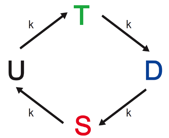
1. Using mass action kinetics, write down a three-dimensional system of differential equations describing this system, assuming that the total amount of KaiC, \(C_\mathrm{tot} = T + U + D + S\), is constant. I.e., write down a system of ODEs for \(T\), \(D\), and \(S\). Assume that $C_:nbsphinx-math:mathrm{tot} = $3.4 µM and \(k = 0.116\text{ h}^{-1}\).

2. Show that there is a unique fixed point and solve for it.

3. Determine the stability of the fixed point using linear stability analysis.

4. Numerically solve for the dynamics of the system from three different initial conditions for a total time of 200 hours. Plot the resulting trajectories.

5. Plot the total phosphorylation of KaiC (T + D + S) versus time for each of the three initial conditions. Explain intuitively why the dynamics have this form, and why this scheme does not appear to generate self-sustaining oscillations. Would you expect the system to behave differently if there were only one molecule of KaiC?

b) Now consider the same system with feedback mediated by KaiA and KaiB.

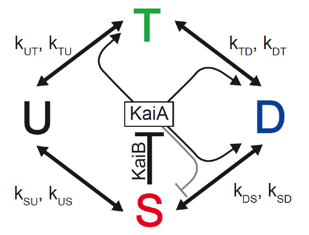
We define \(k_\mathrm{XY}\) as the mass action rate constant (which depends indirectly on S and on the concentration of KaiA, \(A\)) for the conversion from phosphoform X to phosphoform Y. E.g., the rate of conversation from D to S is \(k_\mathrm{DS} D\). We take these constants to be of the following form.

\begin{align} k_\mathrm{XY} &= k^{\text{basal}}_\mathrm{XY} + k^A_\mathrm{XY}\,\frac{A_\mathrm{act}}{A_\mathrm{act}+K_{1/2}}, \end{align}

where

\begin{align} A_\mathrm{act} &= \text{max}\{ 0, A_\mathrm{tot}-2S \} . \end{align}

The constants \(C_\mathrm{tot}\), \(A_\mathrm{act}\), \(k^{\text{basal}}_\mathrm{XY}\), \(k^\mathrm{a}_\mathrm{XY}\), and \(K_{1/2}\) are given in the following table.

Parameter	Value	Units
\(k^{\text{basal}}_\mathrm{UT}\)	0
\(k^{\text{basal}}_\mathrm{TD}\)	0
\(k^{\text{basal}}_\mathrm{SD}\)	0
\(k^{\text{basal}}_\mathrm{US}\)	0
\(k^{\text{basal}}_\mathrm{TU}\)	0.21	h\(^{-1}\)
\(k^{\text{basal}}_\mathrm{DT}\)	0
\(k^{\text{basal}}_\mathrm{DS}\)	0.31	h\(^{-1}\)
\(k^{\text{basal}}_\mathrm{SU}\)	0.11	h\(^{-1}\)
\(k^\mathrm{a}_\mathrm{UT}\)	0.479077	h\(^{-1}\)
\(k^\mathrm{a}_\mathrm{TD}\)	0.212923	h\(^{-1}\)
\(k^\mathrm{a}_\mathrm{SD}\)	0.505692	h\(^{-1}\)
\(k^\mathrm{a}_\mathrm{US}\)	0.0532308	h\(^{-1}\)
\(k^\mathrm{a}_\mathrm{TU}\)	0.0798462	h\(^{-1}\)
\(k^\mathrm{a}_\mathrm{DT}\)	0.173	h\(^{-1}\)
\(k^\mathrm{a}_\mathrm{DS}\)	-0.319385	h\(^{-1}\)
\(k^\mathrm{a}_\mathrm{SU}\)	-0.133077	h\(^{-1}\)
\(K_{1/2}\)	0.43	µM
\(A_\mathrm{tot}\)	1.3	µM
\(C_\mathrm{tot}\)	3.4	µM

1. Write down a the system of ODEs describing this system. Numerically solve them for three different initial conditions of your choosing and plot the result. Make sure that your initial conditions \((T_0, D_0, S_0)\) respect the fact that \(T_0 + D_0 + S_0 \leq C_\mathrm{tot}\). Make sure you integrate long enough to observe the dynamics (200 hours for dimensional units should work).

2. Plot total concentration of phosphorylated KaiC (\(T + D + S\)) versus time for each of the three initial conditions.

3. What is the period of the oscillator? Does it depend on the initial conditions? Why or why not?

4. Why do the initial (transient) dynamics differ depending on initial conditions?

c) A key characteristic of circadian clocks is their so-called phase response curve (PRC), which describes how the phase of the clock changes in response to a stimulus/perturbation such as exposure to light for a defined duration. A PRC is a plot of the change in phase of the clock (\(y\)-axis) versus the phase (subjective time) at which the perturbation is applied (\(x\)-axis). The phase change is evaluated by comparing the phase of the perturbed clock to the phase expected in the absence of perturbation several periods after the perturbation to allow the phase of the perturbed clock to stabilize.

1. For the KaiABC system with feedbacks, apply a perturbation described by \(\delta T = \delta D = \delta S = -0.05\) µM at each hour of the day, that is for 24 different times evenly spaced within [103.5 h, 103.5 hours \(+ T\)), where \(T\) is the period you determined in 3b(iii). (Note that a given system is perturbed only once; you need to run 24 different simulations.) Calculate the trajectories of each of the perturbed systems for at least six periods following the perturbation. Also, calculate the trajectory of an unperturbed clock for at least seven periods following 103.5 hours. Plot the total phosphorylation for the 1st, 6th, 12th, and 18th perturbations versus time, for \(t = [100, 200]\). On the same plot, show the total phosphorylation of the unperturbed clock over the same time period.

2. Now calculate and plot the phase response curve for those 24 perturbations. Define the time at which the perturbation is applied as \(24\times (t_\mathrm{perturb}-t_\text{preceding peak})/T\). Here, \(t_\mathrm{perturb}\) is the time at which the perturbation is applied, \(t_\text{preceding peak}\) is the time of the last peak of total phosphorylation immediately preceding \(t_\mathrm{perturb}\), and \(T\) is the period of the oscillator. The time should lie in the interval [0 h, 24 h). (This formula normalizes time to that of an idealized 24-hour clock, resulting in a measure called circadian time [CT], which is standard in the field.) Define the phase change after perturbation, measured in the CT shift of the total phosphorylation peak, such that it lies in the interval [-12 h, +12 h). To determine the phase change, consider the phase of the perturbed oscillator beginning \(5T\) after perturbation compared to that of the unperturbed oscillator. Match the trajectories plotted in 3c(i) to their circadian times.

3. Describe the implications of this PRC for you if you were a cyanobacterium traveling from Los Angeles to Beijing via a Star Trek-style (instantaneous) transporter. The time in Beijing is 15 hours ahead of the time in Los Angeles; in the date-agnostic PRC in 3c(ii), in which phase changes lie in [-12 h, 12 h), this time difference would be equivalent to a 9-hour phase delay (-9 h). If you could perturb your clock with perturbation \(\delta\) once per day, and the phase change were instantaneous (for the sake of simplicity), describe a scheme for synchronizing your circadian clock with Beijing time.