20. Lateral Inhibition: Spontaneous symmetry allows spontaneous developmental patterning
Design principle
Local interactions between cells can lead to globally-structured spatial patterns
cis-inhibition in the Notch pathway accelerates pattern formation
The instability of a homogenous steady state is a requirement for spontaneous pattern formation
Techniques
Modeling a spatial grid of interacting cells
Simulating and visualizing ODE systems on a grid
References
[1]:
# Colab setup ------------------
import os, sys, subprocess
if "google.colab" in sys.modules:
cmd = "pip install --upgrade biocircuits colorcet watermark"
process = subprocess.Popen(cmd.split(), stdout=subprocess.PIPE, stderr=subprocess.PIPE)
stdout, stderr = process.communicate()
# ------------------------------
import numpy as np
import scipy.integrate
import scipy.optimize
import random
import biocircuits
import bokeh.plotting
import bokeh.io
from bokeh.models import HexTile, MultiLine, Line, Text, Plot, ColorBar, LogColorMapper, ColumnDataSource
import colorcet
import matplotlib
import matplotlib.pyplot as plt
from mpl_toolkits.mplot3d import Axes3D
%matplotlib inline
%config InlineBackend.figure_format = "retina"
# Set to True to have fully interactive plots with Python;
# Set to False to use pre-built JavaScript-based plots
interactive_python_plots = False
notebook_url = "localhost:8888"
bokeh.io.output_notebook()
Development involves spatial patterning of cell fates
In Chapter 14, we discussed the role of cellular differentiation in multicellular development. But multiple cell types alone do not an organism make. It is just as essential that these cell types be spatially organized into body plans and morphologies.
The hair cells on your skin are spaced out at fairly regular intervals that vary in overall density from place to place on your body. There is also a consistent topological organization, with skin enveloping skeleton and interior organs, each with its own structurally and functionally distinct layers.
A beautiful example of spatial patterning occurs in sensory cell development, as one can see with sensor bristles in the inner ear of a developing chick (left) and hair cells from the dorsal thorax of a fruit fly (right). In both cases, patterning defects have functional consequences for the organism, either through impaired hearing in the ear example or through altered aerodynamic properties that could affect flight in the hair cell example. (At the same time, it is important to emphasize that natural spatial patterning processes, such as the generation of a checkerboard array of sound-sensing hairs in the inner ear, are more complex, than the minimal lateral inhibition models we consider below.)
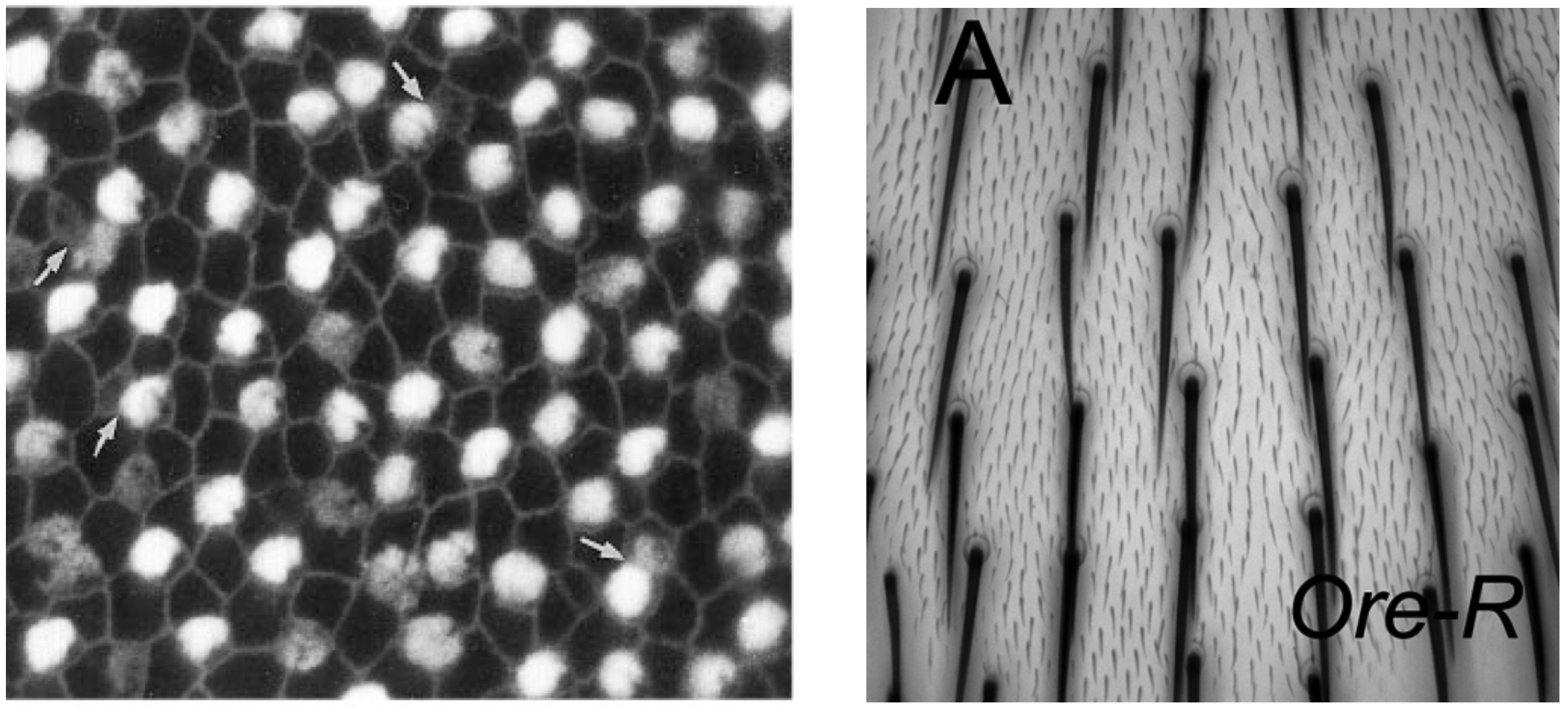
Images from Goodyear and Richardson 1997, J. Neurosci. (left), Lu and Adler 2015, PLoS One (right)
How do cells interact with one another to consistently and precisely self-organize in this way? More generally, can the circuit-level framework developed in previous chapters help us understand multicellular patterning?
To achieve checkerboard patterning, cells need a juxtacrine signaling mechanism to communicate with their neighbors, as well as a circuit that couples intercellular communication with other regulatory interactions.
The Notch-Delta pathway allows juxtacrine communication between neighboring cells
The Notch pathway is the preeminent example of juxtacrine signaling. It is involed in diverse physiological and developmental patterning processes, including the inner-ear and hair cell examples shown above. Notch pathway ligands, known as Delta and Jagged (or Serrate), and Notch receptors are all single-pass transmembrane proteins expressed on the surface of cells. A Notch receptor on one cell can bind to a Delta or Jagged ligand on an adjacent cell. Subsequently, mechanical force generated by endocytosis of the ligand in the signal sending cell leads to the cleavage of the Notch receptor and the consequent release of its intracellular domain (NICD) within the cell. Once released, the NICD translocates to the nucleus, where it activates transcription of Notch pathway target genes.
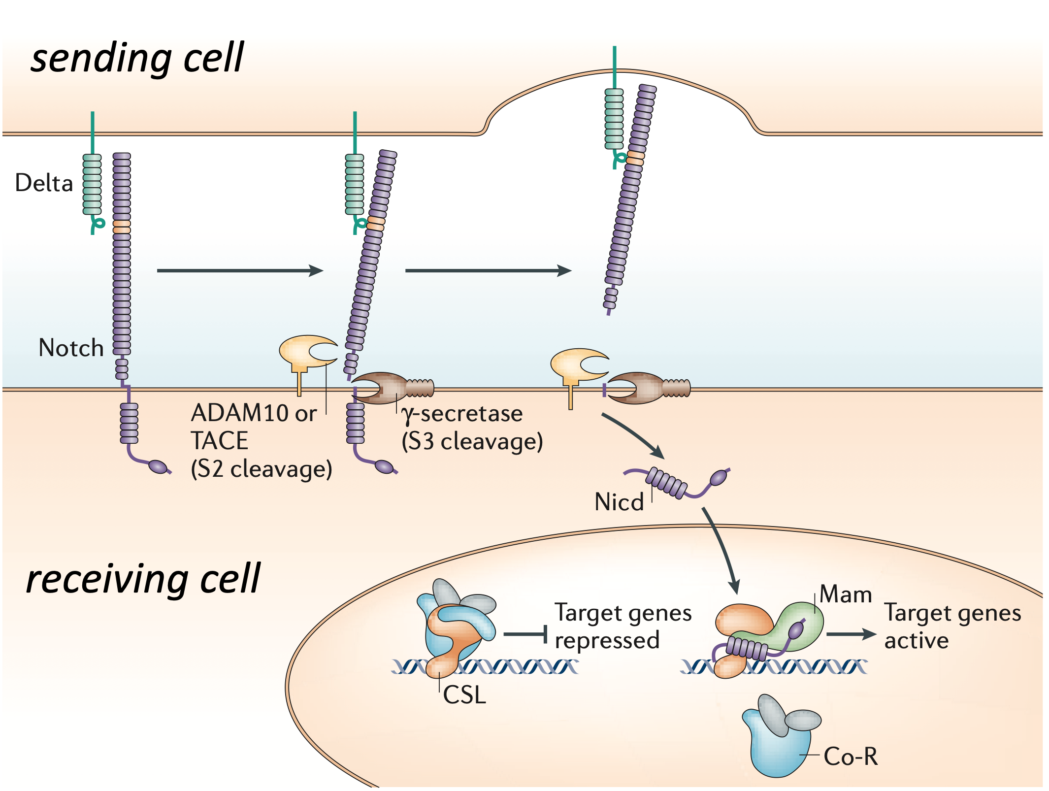
Image adapted from (S. Bray, Nat. Rev. Mol. Cell Bio., 2006)
Historically, the names of Notch receptors and ligands come from pattern-disrupting phenotypes observed in mutants. Notch mutations produce characteristic notches in fly wings, first observed in 1914, while Delta mutations lead to expansion of wing veins to produce formations resembling a river delta.
Note: This is the simplified “classic” view of Notch signaling. We now know that the system is more complicated, and more interesting. Ligands and receptors can interact in the same cell (in “cis”) as well as between cells (in “trans”). And certain ligand-receptor interactions can be inhibitory rather than activating. This repertoire of interactions allows a richer spectrum of patterning behaviors. We will discuss implications of inhibitory cis interactions below.
Lateral inhibition circuits enable checkerboard patterning
Now that we have a signaling pathway in our pocket, how can we use it to create patterns?
In this chapter we will study lateral inhibition, a type of circuit that can, under appropriate conditions, produce spontaneous checkerboard patterning in a field of cells. We will analyze a simplified model of lateral inhibtiion patterning. This model does not seek to represent any particular biological system precisely, but is inspired by features observed in multiple biological contexts, including:
A homogeneous initial condition, in which each cell has an equal potential of becoming one or the other final cell type.
A final pattern comprising a checkerboard of alternating cell types with fine-grain (close to single-cell) spatial resolution.
The ability to form a pattern spontaneously without external signals or cues. This is called spontaneous symmetry breaking.
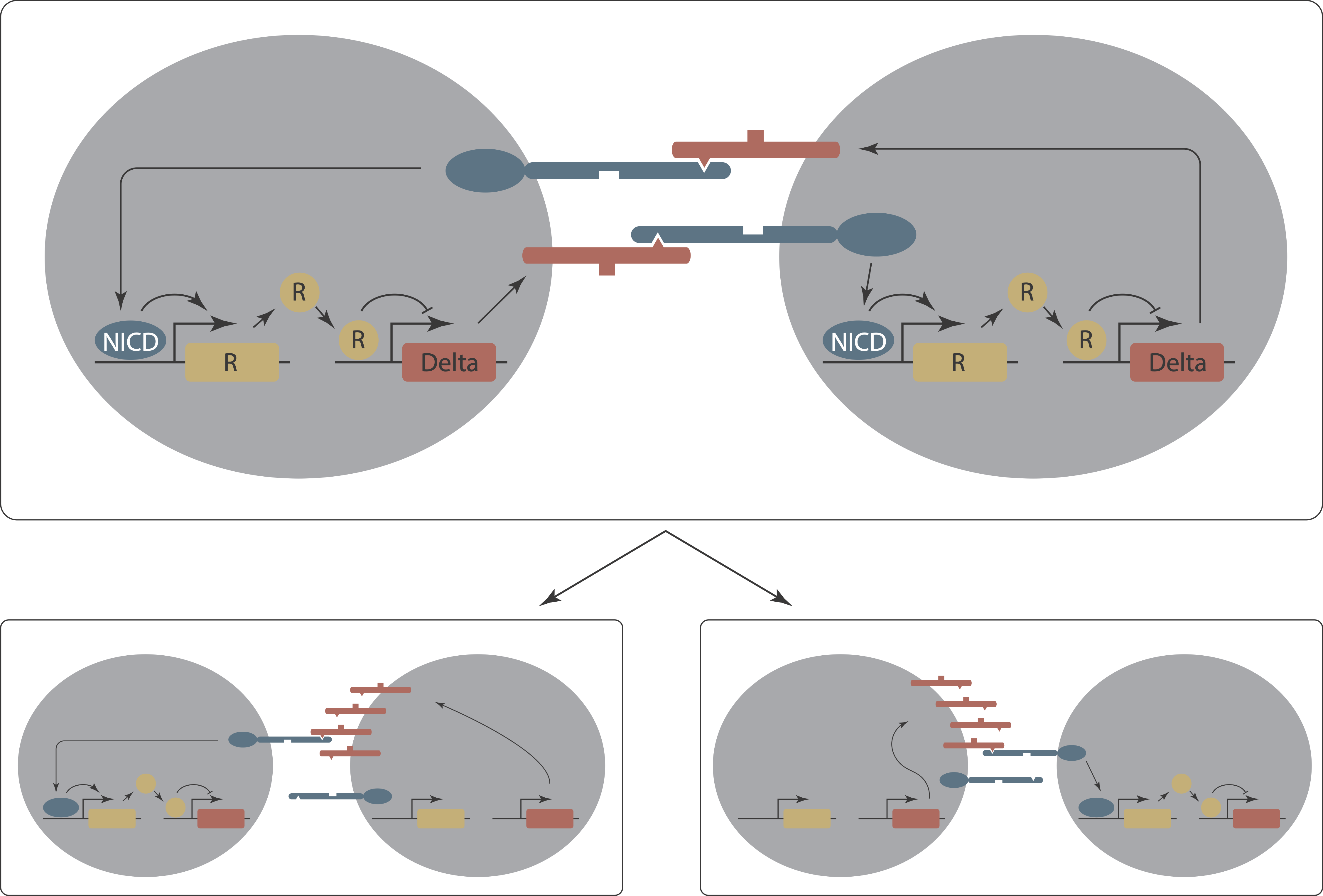
Sprinzak et al. (2011, PLoS Computational Biology) developed a mathematical model of lateral inhibition patterning through Notch signaling. This model, building on previous work, exhibits all three of the features listed above. Lateral inhibition occurs through an intercellular positive feedback loop in which a cell receiving a Notch signal downregulates Delta expression. This in turn reduces the amount of signaling received by neighboring cells. Thus, once a pattern has formed, a cell with high levels of ligand can effectively induce signaling and suppress ligand production in its neighbors.
To understand how this works, consider a minimal system of just two interacting cells. The intercellular positive feedback loop is a bit like the toggle switch we encountered earlier. This time, however, it couples cells together. As a result, a two-cell system—in the right regime—can be bistable, with the two stable states representing ones in which one cell or the other makes high levels of ligand. Critically—again, in the right regime—states in which the two cells have the same concentrations of ligand are unstable.
Now let’s take the circuit into a two-dimensional field of cells. Again, we assume each cell begins with a roughly equal concentration of Notch and Delta on its surface. We will see that this system can reach a stable patterned state, in which cells with high Delta are surrounded by cells with low Delta expression. The stable of the pattern relies on continuous signaling between the cells—if you could remove a low-Delta cell from the pattern and isolate it, without neighbors, it would cease receiving signals, and therefore re-express Delta.
In such a lattice, patterning occurs spontaneously, as shown in the simulation below. Here, each hexagon in the grid represents a single cell and the two colors represent distinct gene expression states.
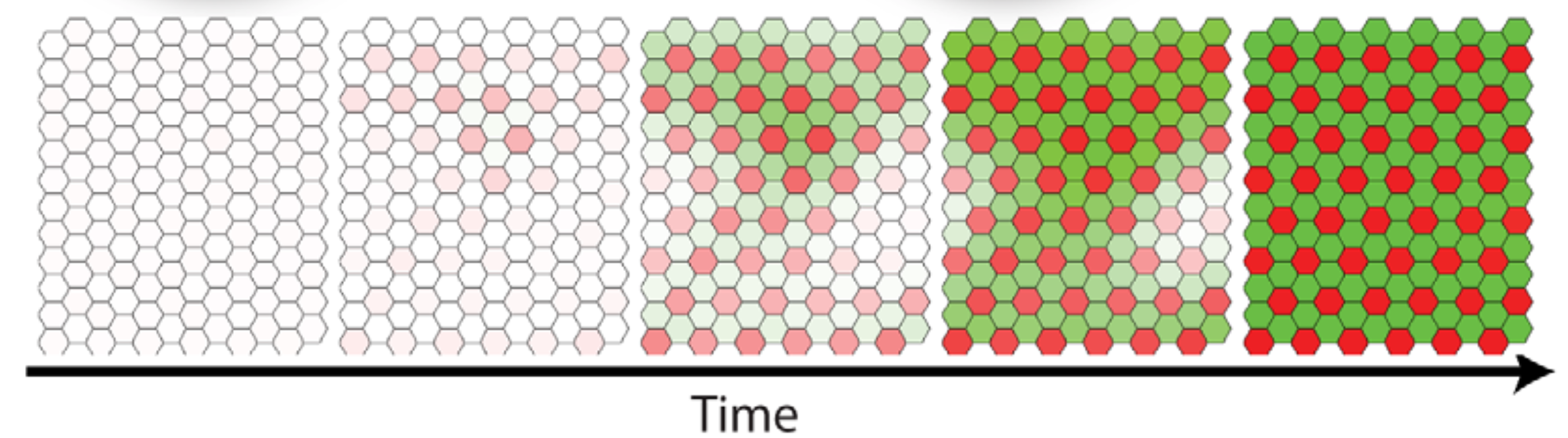
Image from Sprinzak et al. 2011, PLoS Comp. Bio.
In the next section, we will write down the model that produces this dynamic patterning process.
ODEs describe the lateral inhibition system:
Unlike the models we have analyzed so far in this course, this system requires us to keep track of the concentrations of Notch and Delta in every individual cell in a population, and only allows interactions between Notch and Delta molecules that belong to neighboring cells. This is the first time we explicitly deal with spatial organization.
Thankfully, we can incorporate this extra information within the mathematical framework of ODEs. We simply need a lot more of them! We write down one ODE for each protein concentration in each cell.
We begin with the molecular binding reactions. When a Notch receptor on cell \(i\) interacts with a Delta ligand on a neighboring cell \(j\), the two components can bind reversibly to form a bound complex \(T_{ij}\). From this bound state, the intracellular domain of Notch can be cleaved, producing the active signal species \(S_i\) inside the receiver cell. Coincident with this event, both the remainder of the Notch receptor and the Delta ligand on cell are withdrawn back inside the sender cell, so that they no longer exist on the cell membrane and therefore cannot interact with other species. The reaction system governing this process is therefore
\begin{align} N_i + D_j \rightleftharpoons T_{ij} \rightarrow S_i, \end{align}
Here, formation and disassociation of \(T_{ij}\) occur with rate constants \(k_D^+\) and \(k_D^-\), respectively, and \(S_i\) is produced through an irreversible cleavage reaction with rate constant \(k_S\).
How does Notch signaling regulate Delta? Notch is known to activate expression of a set of bHLH transcription factors, which in turn regulate other target genes. Here, we will assume that \(S_i\) acts as a transcriptional activator of a secondary intracellular regulatory molecule \(R_i\) that can, in turn repress Delta in the same cell.
With these assumptions, we can write out the full ODE system. First, let’s return to the simple case of only two cells, labeled \(i\) and \(j\). The ODEs for cell \(i\) are then,
\begin{align} \frac{\mathrm{d}N_i}{\mathrm{d}t} &= \beta_N - \gamma_N N_i - \left( k_D^+ N_iD_j - k_D^- T_{ij}\right) \\ \frac{\mathrm{d}D_i}{\mathrm{d}t} &= \beta_D \frac{1}{1 + (R_i/K_D)^{n_D}} - \gamma_D D_i - \left( k_D^+ N_jD_i - k_D^- T_{ji}\right) \\ \frac{\mathrm{d}T_{ij}}{\mathrm{d}t} &= k_D^+ N_iD_j - k_D^- T_{ij} - k_S T_{ij} \\ \frac{\mathrm{d}S_i}{\mathrm{d}t} &= k_S T_{ij} - \gamma_S S_i \\ \frac{\mathrm{d}R_i}{\mathrm{d}t} &= \beta_R \frac{(S_i/K_R)^{n_R}}{1 + (S_i/K_R)^{n_R}} - \gamma_R R_i. \end{align}
A similar set of five ODEs describes the species \(N_j,D_j, T_{ji}, S_j, R_j\) in the other cell, for a total of ten ODEs in the two-cell system.
We will now make a quasi-steady-state assumption that the binding and cleavage events involved in the formation of \(T_{ij}\) and \(S_i\) are fast enough to be approximately at equilbirium over the longer timescales of gene expression dynamics. Thus,
\begin{align} T_{ij} &= \frac{k_D^+ N_iD_j}{k_D^- + k_S}, \\ S_i &= \frac{k_S}{\gamma_S} T_{ij} = \frac{1}{\gamma_S}\frac{k_S k_D^+}{k_D^- + k_S} N_iD_j \end{align}
We can define \(k_t \equiv (k_D^- + k_S)/k_S k_D^+\) for notational simplicity and substitute the above expressions into our original ODE system to obtain
\begin{align} \frac{\mathrm{d}N_i}{\mathrm{d}t} &= \beta_N - \gamma_N N_i - \frac{N_i D_j}{k_t} \\ \frac{\mathrm{d}D_i}{\mathrm{d}t} &= \beta_D \frac{1}{1 + (R_i/K_D)^{n_D}} - \gamma_D D_i - \frac{D_i N_j}{k_t} \\ \frac{\mathrm{d}R_i}{\mathrm{d}t} &= \beta_R \frac{\left(\frac{N_i D_j}{\gamma_S k_t K_R}\right)^{n_R}}{1 + \left(\frac{N_i D_j}{\gamma_S k_t K_R}\right)^{n_R}} - \gamma_R R_i \end{align}
In order to reduce the parameter complexity of the model, we will further assume that Notch and Delta are degraded at similar rates (\(\gamma \equiv \gamma_N = \gamma_D\)).
As before, we will also nondimensionalize the system, with \(\tilde{t} \leftarrow \gamma_R t\), \(\tilde{N_i} \leftarrow N_i/\gamma k_t\), \(\tilde{D_i} \leftarrow D_i/\gamma k_t\), \(\tilde{R_i} \leftarrow R_i/K_D\), to obtain the nondimensional system (with tildes dropped):
\begin{align} \tau \frac{\mathrm{d}N_i}{\mathrm{d}t} &= \beta_N - N_i - N_i D_j \\ \tau \frac{\mathrm{d}D_i}{\mathrm{d}t} &= \beta_D \frac{1}{1 + R_i^{n_D}} - D_i - N_j D_i \\ \frac{\mathrm{d}R_i}{\mathrm{d}t} &= \beta_R \frac{\left(N_i D_j / k_{RS}\right)^{n_R}}{1 +\left(N_i D_j / k_{RS}\right)^{n_R} } - R_i \end{align}
where we have defined new nondimensional parameters \(\tau \equiv \gamma_R/\gamma\), \(\tilde{\beta_N} \equiv \beta_N / \gamma^2 k_t\), \(\tilde{\beta_D} \equiv \beta_D/\gamma^2 k_t\), \(\tilde{\beta_R} \equiv \beta_R/\gamma_R K_D\), and \(k_{RS} \equiv K_R \gamma_S / \gamma^2 k_t\).
Note that this is a system of six ODEs, with an equivalent set of three ODEs for \(N_j\), \(D_j\), and \(R_j\) that follow the above format.
Simulating the 2-cell system:
Now that we have have written down our model, let’s solve it to see how it performs. Since we can write down all the equations manually, we can use the standard techniques for numerical solution of a system of ODEs that we have covered previously in the course.
[2]:
def LI_2cell_rhs(x, t, betaN, betaD, betaR, nD, nR, kRS, tau):
Ni, Di, Ri, Nj, Dj, Rj = x
return np.array(
[
(betaN - Ni - Ni*Dj)/tau,
(betaD/(1+Ri**nD) - Di - Nj*Di)/tau,
betaR*(Ni*Dj)**nR / (kRS**nR + (Ni*Dj)**nR) - Ri,
(betaN - Nj - Nj*Di)/tau,
(betaD/(1+Rj**nD) - Dj - Ni*Dj)/tau,
betaR*(Nj*Di)**nR / (kRS**nR + (Nj*Di)**nR) - Rj,
]
)
# Parameters (from Sprinzak et al)
betaN = 10
betaD = 100
betaR = 1e6
nD = 1
nR = 3
kRS = 3e5 ** (1/nR)
tau = 1
# initial conditions
Ni0_slider = bokeh.models.Slider(title="Log Initial Ni", start=-3, end=3, step=0.1, value=1)
Di0_slider = bokeh.models.Slider(title="Log Initial Di", start=-3, end=3, step=0.1, value=-3)
Nj0_slider = bokeh.models.Slider(title="Log Initial Nj", start=-3, end=3, step=0.1, value=1)
Dj0_slider = bokeh.models.Slider(title="Log Initial Dj", start=-3, end=3, step=0.1, value=-2.9)
nR_slider = bokeh.models.Slider(title="Cooperativity (nR)", start=0.1, end=10, step=0.1, value=3)
x0 = [10**Ni0_slider.value,
10**Di0_slider.value,
0,
10**Nj0_slider.value,
10**Dj0_slider.value,
0]
# Solve ODEs
t = np.linspace(0, 20, 1000)
args = (betaN, betaD, betaR, nD, nR_slider.value, kRS, tau)
x = scipy.integrate.odeint(LI_2cell_rhs, x0, t, args=args)
x = x.transpose()
cds = bokeh.models.ColumnDataSource(data=dict(t=t, Ni=x[0,:], Di=x[1,:], Ri=x[2,:],
Nj=x[3,:], Dj=x[4,:], Rj=x[5,:]))
# Set up the plots
pN = bokeh.plotting.figure(
frame_width=275, frame_height=150,
x_axis_label="dimensionless time",
y_axis_label="dimensionless\nNotch concentration", y_axis_type="log",
)
pD = bokeh.plotting.figure(
frame_width=275, frame_height=150,
x_axis_label="dimensionless time",
y_axis_label="dimensionless\nDelta concentration", y_axis_type="log",
)
pR = bokeh.plotting.figure(
frame_width=275, frame_height=150,
x_axis_label="dimensionless time",
y_axis_label="dimensionless\nReporter concentration", y_axis_type="log",
)
pN.line(source=cds, x="t", y="Ni", color="blue", width=3, legend_label="Cell i")
pN.line(source=cds, x="t", y="Nj", color="orange", width=3, legend_label="Cell j")
pD.line(source=cds, x="t", y="Di", color="blue", width=3, legend_label="Cell i")
pD.line(source=cds, x="t", y="Dj", color="orange", width=3, legend_label="Cell j")
pR.line(source=cds, x="t", y="Ri", color="blue", width=3, legend_label="Cell i")
pR.line(source=cds, x="t", y="Rj", color="orange", width=3, legend_label="Cell j")
LI_2cell_layout = bokeh.layouts.row(
bokeh.layouts.column(
pN,
pD,
pR,
),
bokeh.layouts.column(
Ni0_slider,
Di0_slider,
Nj0_slider,
Dj0_slider,
nR_slider,
width=150,
)
)
# Display
if interactive_python_plots:
# Set up callbacks
def _callback(attr, old, new):
x0 = [10**Ni0_slider.value,
10**Di0_slider.value,
0,
10**Nj0_slider.value,
10**Dj0_slider.value,
0]
args = (betaN, betaD, betaR, nD, nR_slider.value, kRS, tau)
x = scipy.integrate.odeint(LI_2cell_rhs, x0, t, args=args)
x = x.transpose()
cds.data = dict(t=t, Ni=x[0,:], Di=x[1,:], Ri=x[2,:], Nj=x[3,:], Dj=x[4,:], Rj=x[5,:])
Ni0_slider.on_change("value", _callback)
Di0_slider.on_change("value", _callback)
Nj0_slider.on_change("value", _callback)
Dj0_slider.on_change("value", _callback)
nR_slider.on_change("value", _callback)
# Build the app
def LI_2cell_app(doc):
doc.add_root(LI_2cell_layout)
bokeh.io.show(LI_2cell_app, notebook_url=notebook_url)
else:
Ni0_slider.disabled = True
Di0_slider.disabled = True
Nj0_slider.disabled = True
Dj0_slider.disabled = True
nR_slider.disabled = True
# Build layout
LI_2cell_layout = bokeh.layouts.row(
bokeh.layouts.column(
pN,
pD,
pR,
),
bokeh.layouts.column(
bokeh.layouts.column(
Ni0_slider,
Di0_slider,
Nj0_slider,
Dj0_slider,
width=150
),
bokeh.models.Div(
text="""
<p>Sliders are inactive. To get active sliders, re-run notebook with
<font style="font-family:monospace;">fully_interactive_plots = True</font>
in the first code cell.</p>
""",
width=250,
),
)
)
bokeh.io.show(LI_2cell_layout)
These plots show that the two-cell system can evolve into anti-correlated states, in which each cell takes on either high or low Delta expression. When the initial Notch concentrations of the two cells are equal, this divergence follows a “winner-takes-all” process where the cell that starts with a higher Delta concentration ends up in the high-Delta state.
By using the sliders above to alter the initial values of the Notch concentration, you can see that the full relationship is a bit more subtle. Is it always guaranteed that the two cells will end up in divergent cell states? No— try moving around the slider for the \(n_R\) parameter to see how the system behaves both in regions of low ultrasensitivity and in regimes of high ultrasensitivity. Overall, we see that cells can reach opposite states, which is a prerequisite for patterning. However, this behavior is not guaranteed for all parameters.
Expanding beyond a two-cell system
The model demonstrates that lateral inhibition can produce opposite fates in two neighboring cells. What happens when we take this model beyond two cells to a whole two-dimensional field of cells? In a field of cells, a Notch receptors on cell \(i\), \(N_i\), can interact with Delta ligands on multiple adjacent cells, \(D_j\), to form a variety of distinct \(T_{ij}\) complexes. All of these complexes can then contribute to the formation of \(S_i\) within the receiver cell. Thus,
\begin{align} S_i = \frac{k_S}{\gamma_S} \sum_{j=]i[ } T_{ij} = \frac{1}{\gamma_S}\frac{k_S k_D^+}{k_D^- + k_S}\sum_{j=]i[ } N_iD_j. \end{align}
Here, the notation \(\sum_{j = ]i[}\) means the index \(j\) is iterated over all cells that are adjacent to cell \(i\) (but not including \(i\) itself), and the resulting set is summed together.
Carrying this through the simplifcations and nondimensionalizations given above, we obtain the following nondimensionalized ODE system to accomodate arbitray spatial arrangements of cells:
\begin{align} \tau \frac{\mathrm{d}N_i}{\mathrm{d}t} &= \beta_N - N_i - \sum_{j = ]i[} N_i D_j \\ \tau \frac{\mathrm{d}D_i}{\mathrm{d}t} &= \beta_D \frac{1}{1 + R_i^{n_D}} - D_i - \sum_{j = ]i[} N_j D_i \\ \frac{\mathrm{d}R_i}{\mathrm{d}t} &= \beta_R \frac{\left(\sum_{j = ]i[} N_i D_j / k_{RS}\right)^{n_R}}{1 +\left(\sum_{j = ]i[} N_i D_j / k_{RS}\right)^{n_R} } - R_i \end{align}
Note the way that the summations affect the \(T_{ij}\) formation terms in the \(N_i\) and \(D_i\) ODEs. Although the expressions now look quite a bit more complicated with all these sums, we did not add any new parameters to our system. Visually comparing the above ODE system with the previous ODE system for the two-cell system should reveal how the addition of additional neighbors did not change the fundamental nature of a given species’ dynamics.
We now note two features of this model:
First, it can represent the behavior any number of cells by expanding the size of the ODE system— a system of \(i\) cells can be modeled by \(3i\) equations following the above formula. While such a system would be impractical to solve by hand, using numerical approaches we can solve large ODE systems without much additional difficulty.
Second, the model can represent arbitrary geometric arrangements of cells because the assignment of neighbors to each cell is left arbitrary. Thus we could easily switch between, for example, a square or hexagonal lattice, or even the dimensionality of the space, by changing the neighbor-assignment rule for a given cell. However, the fact that the ODEs do not natively encode the neighbor-assignment rule means that we will have to write an additional function to go inside our ODE solver that identifies the appropriate neighbors for a given cell.
In the technical appendix, we show how to simulate the ODEs on a 1-dimensional line of cells and on a hexagonal two-dimensional lattice of cells.
Patterning in one dimension—the “dotted line.”
Let’s expand our two-cell system to a one-dimensional line of cells. In this arrangement, the neighbors of cell \(i\) are cell \(i-1\) and \(i+1\). But remember that we are only simulating a finite number, \(N\), of cells. Cell \(0\) has no leftward neighbor and cell \(N-1\) has no rightward neighbor. (We will use 0-based indexing, like Python does.) Different choices of how to handle these boundaries, shown below, could all be equally valid depending on the situation being modeled.
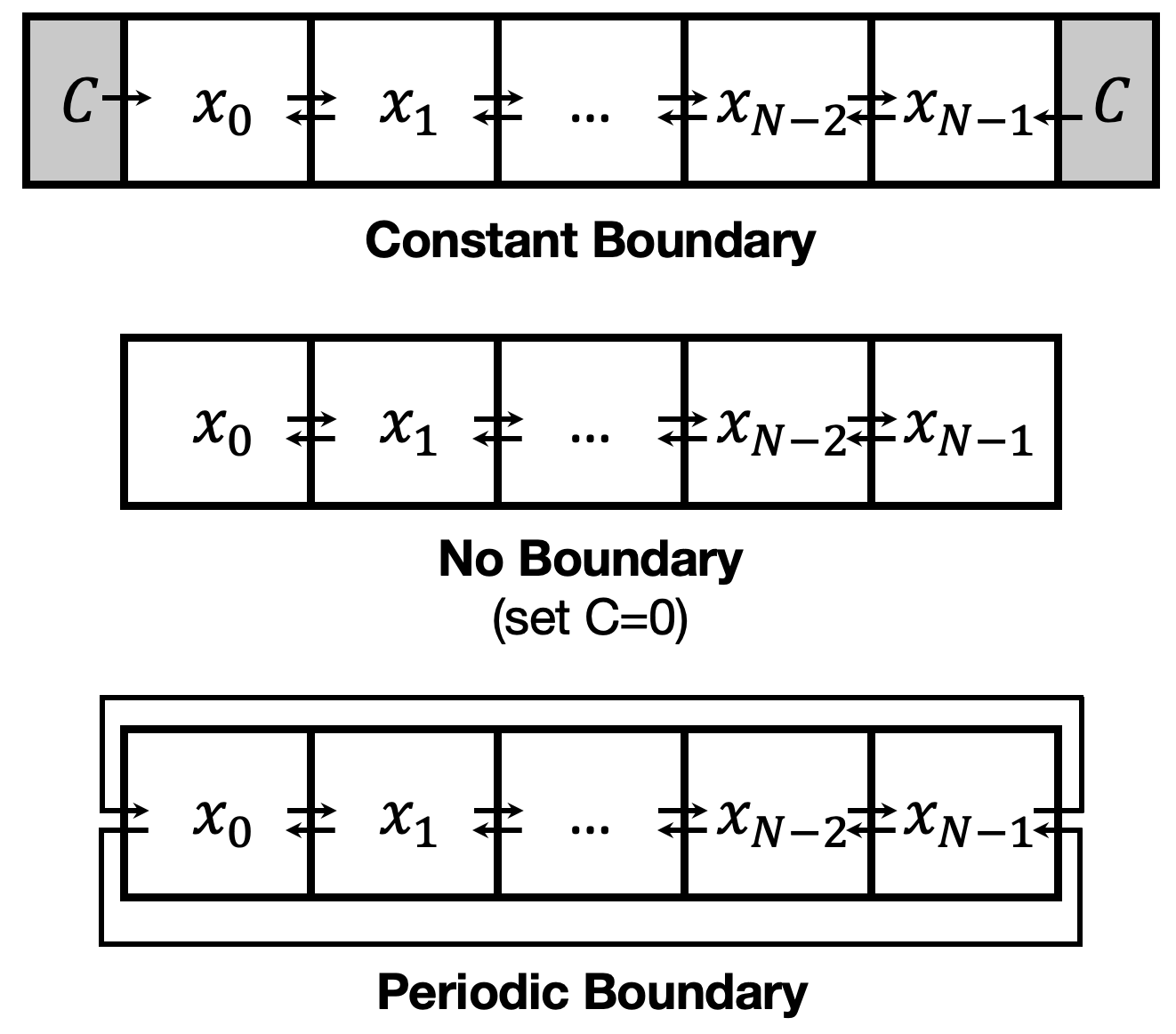
A constant boundary condition might be appropriate when the patterning cells abut against a surrounding population of a different cell type, say one with no Delta expression. A periodic boundary condition, mathematically represents the grid as curving around to loop back on itself, as if it were a loop on the surface of a cylinder, such as cells on the stem of a plant.
Thus for a system of ODEs solved over a spatially-explicit arrangement of cells, we need to specify the following for the problem to be complete: 1. The system’s dynamics within an individual cell (the ODEs) 2. The arrangement of the cells in space, including special rules for the boundaries (the Neighbor Rule)
In the technical appendix (ADD LINK HERE) we show how you can solve a set of ODEs on a lattice of cells.
Numerical solution of the Lateral Inhibition model on a 2D hexagonal lattice
Let’s now consider how we would numerically solve our ODE system on a 2D lattice of hexagonal cells. We choose this particular spatial arrangement because it mirrors how cells are packed in the fruit fly wing. Because the number of equations in the system varies with the number of cells, we cannot hard-code a function that manually writes out every ODE in our system. This would not only be cumbersome, but we would have to write a new ODE function every time we wanted to change the number of cells we are simulating. We will instead write a helper function that our ODE function can call to generate the required neighbor information for an arbitrary cell.
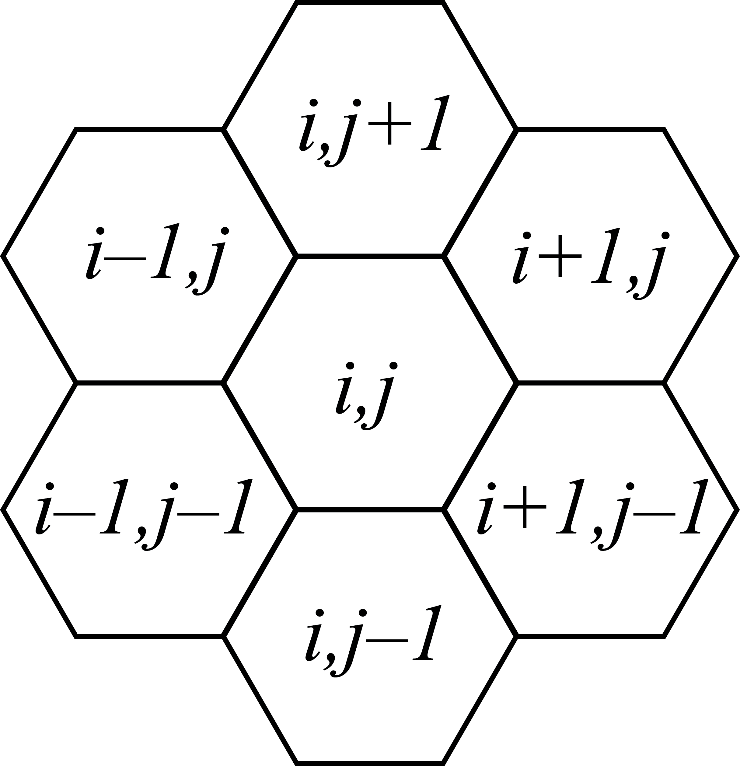
How do we define neighbors in a hexagonal grid? It turns out that a 2-dimensional indexing can fully define the location of a cell in a hexagonal grid, just as it can for a square grid. While in a square grid the four neighbors of cell \((i,j)\) would be the cells \((i+1,j)\), \((i,j-1)\), \((i-1,j)\), and \((i,j+1)\), in a hexagonal grid the six neighbors of cell \((i,j)\) are \((i+1,j)\), \((i+1,j-1)\), \((i,j-1)\), \((i-1,j)\), \((i-1,j+1)\), and \((i,j+1)\). Using this rule we can therefore define a helper function that, given the system’s species concentration vector \(\boldsymbol{x}\) and the cell indices \(i,j\), return the sum of the concentrations of a particular species in all of the neighbors of cell \((i,j)\).
However, our function is not yet complete because we have not specified our boundary conditions. Here we will choose to use periodic boundary conditions, whicih means that in an \(N\times N\) grid of cells, the upper-right-most cell \((N-1,N-1)\) is neighbors with the lower-left-most cell \((0,0)\). While it is possible to hard-code all the edge cases and modify the neighbor rule accordingly within the helper function, doing so would be extremely cumbersome. Instead we will take a more general approach, which is to use modular arthithmetic.
While standard arithmetic performs algebraic operations like addition and multiplication along the real number line, modular arithmetic can be conceptualized as performing these same operations along a circular number line that behaves like a clock. On the face of a 12-hour clock, adding 2 hours to 11:00 doesn’t give 13:00, but rather 1:00. This is equivalent to performing the \(11+2\) operation modulo \(12\), which gives the result of \(1\).
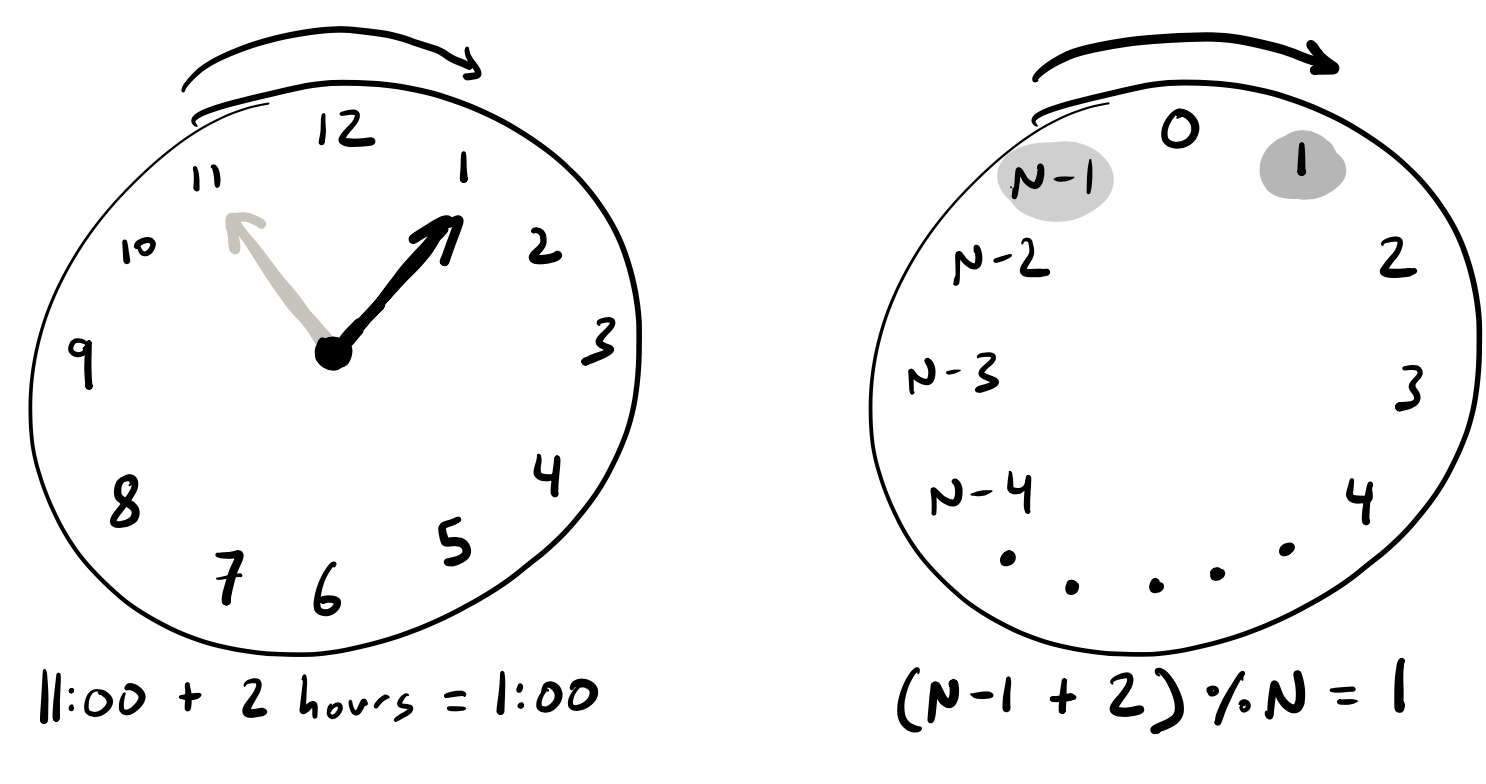
If we apply this concept to our 2D hexagonal grid of cells, we can see that if we perform all of our addition and subtraction operations from our neighbor rule modulo \(N\), then we don’t need to write special cases for our periodic boundary conditions. \(N-1 + 1 = 0\), and \(0 - 1 = N-1\). In Python you can perform modular arithmetic by performing the standard operation and doing the modulo division operation on the modulus number, which is represented by the symbol %. So if
you wanted to code the operation \(2 + 3\) modulo \(4\), then you would write (2+3) % 4.
We have now specified all of the properties required to fully determine the dynamics of our system, but we still need to consider one more thing before we can calculate our numerical solution. In the grid mindset above, we are conceptualizing our cellular grid here as a 2-dimensional grid, our ODE solver scipy.integrate.odeint() can only take a 1-dimensional vector as an argument. This is a common theme that will arise as you use computational methods for your research— you will find that
tools and packages developed by others may not interface with your particular problem in exactly the right way, so you will have to do some work to bridge the gap.
In this case, we will resolve this issue by converting our concentration array back and forth between a one-dimensional form and a three-dimensional form (two spatial dimensions and a third dimension to hold the 3 species concentrations for a given cell) using the np.reshape() operation. This allows us get the best of both worlds by working with the more intuitive multi-dimensional form of the array whenever we are intializing the system or calculating neighbors, but still enabling us to use
the powerful performance of scipy.integrate.odeint().
We are now ready to code up our ODE system for a 2D lattice and solve it! We do so below for a \(12\times 12\) grid, intializing the system at a homogeneous state where all of the cells have the same concentrations of every species, but then adding some independent normally-distributed noise around the nonzero concentrations such that the magnitude of the noise tend to be within 10% of the mean value.
The cell below will take a few seconds to run.
[3]:
# Write helper functions
def get_Djs_hex_periodic(x3, i, j):
r = x3.shape[0]
return x3[(i+1)%r,j,1] + x3[(i+1)%r,(j-1)%r,1] + x3[i,(j-1)%r,1] + x3[(i-1)%r,j,1] + x3[(i-1)%r,(j+1)%r,1] + x3[i,(j+1)%r,1]
def get_Njs_hex_periodic(x3, i, j):
r = x3.shape[0]
return x3[(i+1)%r,j,0] + x3[(i+1)%r,(j-1)%r,0] + x3[i,(j-1)%r,0] + x3[(i-1)%r,j,0] + x3[(i-1)%r,(j+1)%r,0] + x3[i,(j+1)%r,0]
# Write ODE rhs function
def LI_hex_periodic_rhs(x, t, betaN, betaD, betaR, nD, nR, kRS, tau):
"""
Assumes a square NxN grid of cells with hexagonal tiling
and periodic boundary conditions.
"""
# confirm that the reshape procedure worked properly
assert len(x) % 3 == 0
numcells = int(len(x)/3)
numrows = np.sqrt(numcells)
assert numrows % 1 == 0
numrows = int(numrows)
# Reshape the concentration array to 3D
x3 = x.reshape((numrows,numrows,3))
dxdt_3 = np.empty((numrows, numrows, 3))
for i in range(numrows):
for j in range(numrows):
Ni = x3[i,j,0]
Di = x3[i,j,1]
Ri = x3[i,j,2]
Djs = get_Djs_hex_periodic(x3, i, j)
Njs = get_Njs_hex_periodic(x3, i, j)
dxdt_3[i,j,0] = (betaN - Ni - Ni*Djs)/tau
dxdt_3[i,j,1] = (betaD/(1+Ri**nD) - Di - Njs*Di)/tau
dxdt_3[i,j,2] = betaR*(Ni*Djs)**nR / (kRS**nR + (Ni*Djs)**nR) - Ri
# Reshape output array to 1D
dxdt = dxdt_3.reshape(numrows*numrows*3,)
return dxdt
# Parameters
betaN = 10
betaD = 100
betaR = 1e6
nD = 1
nR = 3
kRS = 3e5 ** (1/nR)
tau = 1
numrows = 12
# Define initial conditions
Ni0 = 10
Di0 = 1e-3
Ri0 = 0
# Define noise around the initial condition
Ni0_std = Ni0 / 10 / 2 # 98% of samples will be within 10% of Ni0
Di0_std = Di0 / 10 / 2 # 98% of samples will be within 10% of Di0
x0_3 = np.empty((numrows,numrows,3))
for i in range(numrows):
for j in range(numrows):
x0_3[i,j,0] = np.random.normal(Ni0, Ni0_std)
x0_3[i,j,1] = np.random.normal(Di0, Di0_std)
x0_3[i,j,2] = 0
x0 = x0_3.reshape(numrows*numrows*3,)
# Solve ODEs
tmax = 30
numpoints = 1000
t = np.linspace(0, tmax, numpoints)
args = (betaN, betaD, betaR, nD, nR, kRS, tau)
x = scipy.integrate.odeint(LI_hex_periodic_rhs, x0, t, args=args)
x = x.transpose()
# Reshape output array to convenient shape
x4 = x.reshape((numrows,numrows,3,1000))
[4]:
# Set up plots
pT = bokeh.plotting.figure(
frame_width=375, frame_height=200,
x_axis_label="dimensionless time",
y_axis_label="dimensionless\nconcentration", y_axis_type="log",
x_range = [0, tmax], y_range=[1e-4,1e4],
title="Lateral Inhibition, 12x12 periodic hexagonal grid"
)
pND = bokeh.plotting.figure(
frame_width=250, frame_height=250,
x_axis_label="dimensionless\nNotch concentration", x_axis_type="log",
y_axis_label="dimensionless\nDelta concentration", y_axis_type="log",
x_range=[2e-2, 2e1], y_range=[4e-4, 1e2]
)
# Slider to control time
time_slider = bokeh.models.Slider(title="time index", start=0, end=numpoints-1, step=1, value=650)
# Set up MultiLine Glyph
NDsource = ColumnDataSource(dict(
ts = list(np.tile(t[:time_slider.value], (numrows*numrows,1))),
Ns = list(np.reshape(x4[:,:,0,:time_slider.value], (numrows*numrows, time_slider.value))),
Ds = list(np.reshape(x4[:,:,1,:time_slider.value], (numrows*numrows, time_slider.value))),
Rs = list(np.reshape(x4[:,:,2,:time_slider.value], (numrows*numrows, time_slider.value))),
)
)
Tsource = ColumnDataSource(dict(
ts = list(np.tile(t[:], (numrows*numrows,1))),
Ns = list(np.reshape(x4[:,:,0,:], (numrows*numrows, numpoints))),
Ds = list(np.reshape(x4[:,:,1,:], (numrows*numrows, numpoints))),
Rs = list(np.reshape(x4[:,:,2,:], (numrows*numrows, numpoints))),
)
)
t_cds = ColumnDataSource(dict(curr_t = np.repeat(t[time_slider.value - 1], 2), y=np.array([1e-4,1e4])))
N_glyph = MultiLine(xs="ts", ys="Ns", line_color="blue", line_width=2, line_alpha=.2, syncable=False)
D_glyph = MultiLine(xs="ts", ys="Ds", line_color="red", line_width=2, line_alpha=.2, syncable=False)
R_glyph = MultiLine(xs="ts", ys="Rs", line_color="green", line_width=2, line_alpha=.2, syncable=False)
pT.add_glyph(Tsource, N_glyph)
pT.add_glyph(Tsource, D_glyph)
pT.add_glyph(Tsource, R_glyph)
ND_glyph = MultiLine(xs="Ns", ys="Ds", line_color="black", line_width=2, line_alpha=0.2)
pND.add_glyph(NDsource, ND_glyph)
T_glyph = Line(x="curr_t", y="y", line_color="black", line_width=2)
pT.add_glyph(t_cds, T_glyph)
# Display
if interactive_python_plots:
# Set up callbacks
def _callback(attr, old, new):
t_ls = np.tile(t[:time_slider.value], (numrows*numrows,1))
N_ls = np.reshape(x4[:,:,0,:time_slider.value], (numrows*numrows, time_slider.value))
D_ls = np.reshape(x4[:,:,1,:time_slider.value], (numrows*numrows, time_slider.value))
NDsource.data = dict(
ts = list(t_ls),
Ns = list(N_ls),
Ds = list(D_ls),
# Rs = list(R_ls),
)
t_cds.data = dict(dict(curr_t = np.repeat(t[time_slider.value -1], 2), y=np.array([1e-4,1e4])))
time_slider.on_change("value_throttled", _callback)
LI_hex_tcourse_layout = bokeh.layouts.row(
bokeh.layouts.column(
pT,
time_slider,
),
pND
)
# Build the app
def LI_hex_tcourse_app(doc):
doc.add_root(LI_hex_tcourse_layout)
bokeh.io.show(LI_hex_tcourse_app, notebook_url=notebook_url)
else:
time_slider.disabled=True
LI_hex_tcourse_layout = bokeh.layouts.row(
bokeh.layouts.column(
pT,
time_slider,
),
bokeh.layouts.column(
pND,
bokeh.models.Div(
text="""
<p>Sliders are inactive. To get active sliders, re-run notebook with
<font style="font-family:monospace;">fully_interactive_plots = True</font>
in the first code cell.</p>
""",
width=250,
),
)
)
bokeh.io.show(LI_hex_tcourse_layout)