4a. Numerical solution of FFLs
[1]:
# Colab setup ------------------
import os, sys, subprocess
if "google.colab" in sys.modules:
    cmd = "pip install --upgrade colorcet biocircuits watermark"
    process = subprocess.Popen(cmd.split(), stdout=subprocess.PIPE, stderr=subprocess.PIPE)
    stdout, stderr = process.communicate()
# ------------------------------

import numpy as np
import scipy.integrate

import biocircuits

import colorcet
colors = colorcet.b_glasbey_category10

import bokeh.io
import bokeh.layouts
import bokeh.models
import bokeh.plotting

bokeh.io.output_notebook()
It is useful to write functions to solve for the dynamics of FFLs in response to a step up and a step down to quickly explore the dynamics of the various sub-architectures of the FFL.
As a reminder, the architectures for the various FFLs are shown below.
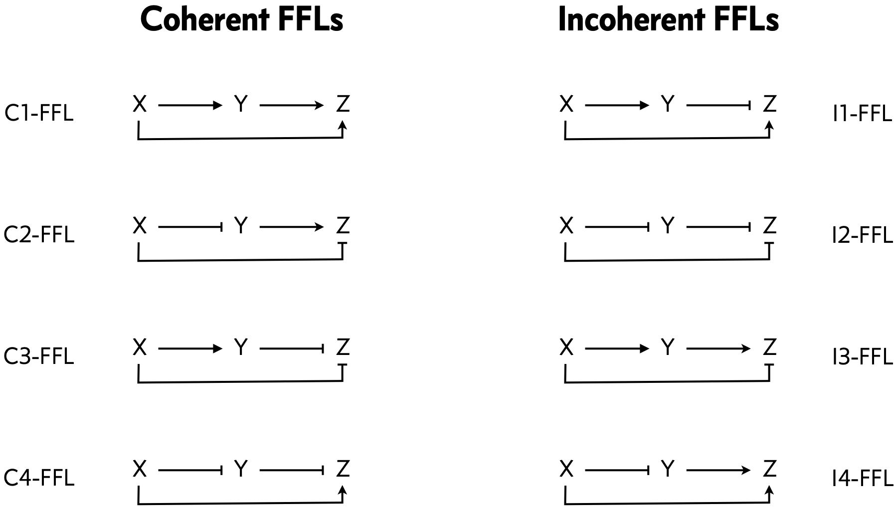
Each architecture may feature AND or OR logic for the regulation of Z by X and Y. As we worked out in the chapter, the dimensionless dynamical equations for an FFL are
\begin{align} \frac{\mathrm{d}y}{\mathrm{d}t} &= \beta\,f_y\left(\kappa x; n_{xy}\right) - y,\\[1em] \gamma^{-1}\,\frac{\mathrm{d}z}{\mathrm{d}t} &= f_z(x, y; n_{xz}, n_{yz}) - z, \end{align}
where the function \(f_y\) specifies how the expression of Y is regulated by the concentration of X and the function \(f_z\) specifies how the expression of Z is regulated by the concentrations of X and Y. We can use the regulatory functions included in the biocircuits when we code up the ODEs for FFLs.
It is convenient to define a function that will give back a function that we can use as the right-hand side we need to specify to scipy.integrate.odeint(). Remember that odeint() requires a function of the form func(yz, t, *args), where yz is an array of length two containing the values of \(y\) and \(z\). For convenience, our function will return a function with call signature rhs(yz, t, x), where x is the value of \(x\) at a given time point.
[2]:
def ffl_rhs(beta, gamma, kappa, n_xy, n_xz, n_yz, ffl, logic):
    """Return a function with call signature fun(yz, x) that computes
    the right-hand side of the dynamical system for an FFL. Here,
    `yz` is a length two array containing concentrations of Y and Z.
    """
    if ffl[:2].lower() in ("c1", "c3", "i1", "i3"):
        fy = lambda x: biocircuits.act_hill(x, n_xy)
    else:
        fy = lambda x: biocircuits.rep_hill(x, n_xy)

    if ffl[:2].lower() in ("c1", "i4"):
        if logic.lower() == "and":
            fz = lambda x, y: biocircuits.aa_and(x, y, n_xz, n_yz)
        else:
            fz = lambda x, y: biocircuits.aa_or(x, y, n_xz, n_yz)
    elif ffl[:2].lower() in ("c4", "i1"):
        if logic.lower() == "and":
            fz = lambda x, y: biocircuits.ar_and(x, y, n_xz, n_yz)
        else:
            fz = lambda x, y: biocircuits.ar_or(x, y, n_xz, n_yz)
    elif ffl[:2].lower() in ("c2", "i3"):
        if logic.lower() == "and":
            fz = lambda x, y: biocircuits.ar_and(y, x, n_yz, n_xz)
        else:
            fz = lambda x, y: biocircuits.ar_or(y, x, n_yz, n_xz)
    else:
        if logic.lower() == "and":
            fz = lambda x, y: biocircuits.rr_and(x, y, n_xz, n_yz)
        else:
            fz = lambda x, y: biocircuits.rr_or(x, y, n_xz, n_yz)

    def rhs(yz, t, x):
        y, z = yz
        dy_dt = beta * fy(kappa * x) - y
        dz_dt = gamma * (fz(x, y) - z)

        return np.array([dy_dt, dz_dt])

    return rhs
To study the dynamics, we will investigate how the circuit responds to a step up in concentration of X, assuming all concentrations are initially zero, and how a circuit at steady state with nonzero concentration of X responds to a step down in X to zero. This case is particularly relevant for a C1-FFL and an I1-FFL, since in the absence of X (and leakage), the steady state levels of both Y and Z are zero. For other FFLs, the steady state concentrations of Y or Z absent X can be nonzero. In this case, you can think of the sudden rise in X being associated also with a sudden rise of effectors that allow Y and Z to turn on.
Now we can write a function to solve the ODEs. Because the steps are discontinuous, we need to solve the ODEs in a piecewise manner. We specify that the step up starts at \(t = 0\), and we will allow the time of the step down to be specified. The magnitude of the step up, \(x_0\) will also be specified.
[3]:
def solve_ffl(beta, gamma, kappa, n_xy, n_xz, n_yz, ffl, logic, t, t_step_down, x_0):
    """Solve an FFL. The dynamics are given by
    `rhs`, the output of `ffl_rhs()`.
    """
    if t[0] != 0:
        raise RuntimeError("time must start at zero.")

    rhs = ffl_rhs(beta, gamma, kappa, n_xy, n_xz, n_yz, ffl, logic)

    # Integrate if we do not step down
    if t[-1] < t_step_down:
        return scipy.integrate.odeint(rhs, np.zeros(2), t, args=(x_0,))

    # Integrate up to step down
    t_during_step = np.concatenate((t[t < t_step_down], (t_step_down,)))
    yz_during_step = scipy.integrate.odeint(
        rhs, np.zeros(2), t_during_step, args=(x_0,)
    )

    # Integrate after step
    t_after_step = np.concatenate(((t_step_down,), t[t > t_step_down]))
    yz_after_step = scipy.integrate.odeint(
        rhs, yz_during_step[-1, :], t_after_step, args=(0,)
    )

    # Concatenate solutions
    if t_step_down in t:
        return np.vstack((yz_during_step[:-1, :], yz_after_step))
    else:
        return np.vstack((yz_during_step[:-1, :], yz_after_step[1:, :]))
Finally, we can write a function to solve and plot the dynamics of an FFL for a unit step.
[4]:
def plot_ffl(
    beta=1.0,
    gamma=1.0,
    kappa=1.0,
    n_xy=1.0,
    n_xz=1.0,
    n_yz=1.0,
    ffl="c1",
    logic="and",
    t=np.linspace(0, 20, 200),
    t_step_down=10.0,
    x_0=1.0,
    normalized=False,
):
    yz = solve_ffl(
        beta, gamma, kappa, n_xy, n_xz, n_yz, ffl, logic, t, t_step_down, x_0
    )
    y, z = yz.transpose()

    # Generate x-values
    if t[-1] > t_step_down:
        t_x = np.array([-t_step_down / 10, 0, 0, t_step_down, t_step_down, t[-1]])
        x = np.array([0, 0, x_0, x_0, 0, 0], dtype=float)
    else:
        t_x = np.array([-t[-1] / 10, 0, 0, t[-1]])
        x = np.array([0, 0, x_0, x_0], dtype=float)

    # Add left part of y and z-values
    t = np.concatenate(((t_x[0],), t))
    y = np.concatenate(((0,), y))
    z = np.concatenate(((0,), z))

    # Normalize if necessary
    if normalized:
        x /= x.max()
        y /= y.max()
        z /= z.max()

    # Set up figure
    p = bokeh.plotting.figure(
        frame_height=175,
        frame_width=550,
        x_axis_label="dimensionless time",
        y_axis_label=f"{'norm. ' if normalized else ''}dimensionless conc.",
        x_range=[t.min(), t.max()],
    )

    # Column data sources
    cds = bokeh.models.ColumnDataSource(dict(t=t, y=y, z=z))
    cds_x = bokeh.models.ColumnDataSource(dict(t=t_x, x=x))

    # Populate glyphs
    p.line(source=cds_x, x="t", y="x", line_width=2, color=colors[0], legend_label="x")
    p.line(source=cds, x="t", y="y", line_width=2, color=colors[1], legend_label="y")
    p.line(source=cds, x="t", y="z", line_width=2, color=colors[2], legend_label="z")

    # Allow vanishing lines by clicking legend
    p.legend.click_policy = "hide"

    return p
We can take this for a spin to see the response of an I1-FFL.
[5]:
# Parameter values
beta = 5
gamma = 1
kappa = 1
n_xy, n_yz = 3, 3
n_xz = 5

# Plot
p = plot_ffl(beta, gamma, kappa, n_xy, n_xz, n_yz, ffl="i1", logic="and")
bokeh.io.show(p)
The functionality of the solve_ffl() and plot_ffl() functions are available in the biocircuits packages as biocircuits.apps.solve_ffl() and biocircuits.apps.plot_ffl(). The biocircuits.apps.plot_ffl() also outputs the ColumnDataSources cds and cds_x that are used in constructing the FFL explorer app, so its API does differ from the function defined above.
Computing environment
[6]:
%load_ext watermark
%watermark -v -p numpy,scipy,bokeh,biocircuits,jupyterlab
Python implementation: CPython
Python version       : 3.10.10
IPython version      : 8.10.0

numpy      : 1.23.5
scipy      : 1.10.0
bokeh      : 3.1.0
biocircuits: 0.1.9
jupyterlab : 3.5.3