7. Amplification of extracellular signals

---

Design principles

• Bifunctional kinases that paradoxically phosphorylate and dephosphorylate their targets enable linear amplification that is robust to total protein copy numbers.

• Biphasic control can be accomplished with paradoxical regulation.

• Kinase cascades can yield both ultrasensitive and graded responses using the same architecture.

Concepts

• Paradoxical regulation

Techniques

• Applying conservation laws to simplify circuit analysis.

---

# Colab setup ------------------
import os, sys, subprocess
if "google.colab" in sys.modules:
    cmd = "pip install --upgrade watermark"
    process = subprocess.Popen(cmd.split(), stdout=subprocess.PIPE, stderr=subprocess.PIPE)
    stdout, stderr = process.communicate()
# ------------------------------

import numpy as np
import scipy.integrate

import bokeh.io
import bokeh.plotting

bokeh.io.output_notebook()

Loading BokehJS ...

Amplifiers: the middle managers of biological circuitry

Cells sense and respond to a variety of external signaling molecules, including protein growth factors and hormones in multicellular organisms, and peptide or small molecule signals in bacteria. They also process internal signals encoded in the states and concentrations of proteins. In many cases, the numbers of molecules being sensed may be much smaller than the number of downstream molecules that need to be activated. For example, an incoming signal may need to ultimately activate thousands of copies of a transcription factor to bind to and activate all of the relevant genomic targets. This requires signal amplification.

One of the most dramatic examples of amplification occurs in the light-sensing cells of the retina, which amplify detection of a single photon into the hydrolysis of 10⁵ cyclic GMP molecules. This event, in turn, leads to a response that blocks more 10⁶ sodium ions from entering the cell over a period of one second. This amplification process is so strong that it can enable conscious perception of single photons (Tinsley, et al., 2016).

Amplifiers play several distinct roles within circuits. Most obviously, they increase the magnitude of signals. Or, in some cases, they can also act as de-amplifiers (called attenuators) to reduce the amplitude of a signal. Second, amplifiers can reshape signals. For example, an ultrasensitive amplifier can allow a system to respond in a switch-like manner when inputs exceed a defined threshold. A third feature of many amplifiers is their ability to convert signals from one molecular form to another, e.g. from protein abundance to protein phosphorylation.

Amplifiers are like middle managers; they take results from one group, extract and emphasize or diminish certain features, and then pass the results along to others in a new form.

In this chapter, we will explore different types of amplifiers based on protein kinases. These phosphorylation-based amplifiers can operate rapidly and directly, entirely at the protein level. They also play key roles in a variety of central biological processes. We note that other classes of systems, such as transcriptional regulation, can also perform amplification functions. We will focus on two of the most important classes of kinase amplifiers: two-component systems in prokaryotes and mitogen-activated protein (MAP) kinase cascades in eukaryotes. We will learn how these amplifiers can operate in a manner that is robust to their own component concentrations and how they can allow tuning of two key properties: gain and sensitivity.

Amplifiers are characterized by their transfer functions

Consider designing a biomolecular sensor module that encodes the concentration of an input signal in the concentration of a target protein. Cells have to do this all the time in order to transmit information about the external environment from sensory components at the periphery of the cell to regulatory components in the interior of the cell. As they convert information from the input to the effector molecule, in a process called signal transduction, they also amplify (or sometimes de-amplify) it, making the effector response larger (or smaller) than the input.

The relationship between the concentration of an input signal, \(x\), and the magnitude of the output response, \(y\), is the transfer function, \(y = f(x)\). Transfer functions have several key features:

• Gain, \(g\), is the multiplier by which an output signal is increased relative to its input, \(g = f(x)/x\). For linear amplifiers, \(g\) is constant, but more generally it will depend on input level, \(x\). Values of \(g\) less than 1 represent de-amplification.

• The derivative of the transfer curve, \(\mathrm{d}f/\mathrm{d}x\), is the change in output produced by a small change in input. For a linear amplifier, this is identical to the gain, \(g\).

• Related to the derivative is the sensitivity, which is logarithmic derivative of the transfer function: \begin{align} \text{sensitivity} = \frac{\mathrm{d}\ln f}{\mathrm{d} \ln x} = \frac{x}{f(x)}\,\frac{\mathrm{d}f}{\mathrm{d}x}. \end{align} Sensitivity quantifies the fractional change in output produced by a fractional change in input. For a linear transfer function the sensitivity is one. Note that a system can be linearly sensitive and still have a high gain. Sensitivity can strongly influence circuit behaviors. For example, in Chapter 3 we saw that ultrasensitive regulation (sensitivity > 1) was required for bistability in both the positive autoregulatory feedback loop and mutual repression toggle switch. On the other hand, we saw in Chapter 5 that incoherent feed-forward loops enable dosage compensation when regulation is linear (\(n=1\)).

To see an example, consider the activating Hill function as a transfer curve:

\begin{align} y = f(x) = \frac{(x/k)^n}{1 + (x/k)^n}. \end{align}

The gain, derivative, and sensitivity are, respectively,

\begin{align} &\mathrm{gain} = \frac{1}{k}\,\frac{(x/k)^{n-1}}{1+(x/k)^n},\\[1em] &\mathrm{derivative} = \frac{1}{k}\,\frac{n (x/k)^{n-1}}{(1+(x/k)^n)^2},\\[1em] &\mathrm{sensitivity} = \frac{n}{1 + (x/k)^n}. \end{align}

These features are plotted below.

A note on terminology. The terms “transfer function,” “gain,” and “sensitivity” all have various meanings among and within the fields of signal processing, controls, and electronics, and even within systems biology. This may cause confusion when reading further about these concepts. We have defined these terms above and will use those definitions throughout this chapter and beyond.

n_slider = bokeh.models.Slider(title="n", name="n", start=1, end=20, step=0.1, value=4)

n = n_slider.value
x = np.logspace(-3, 3, 200)
y = x ** n / (1 + x ** n)

p = bokeh.plotting.figure(
    frame_width=350,
    frame_height=175,
    x_axis_label="x/k",
    x_axis_type="log",
    y_axis_type="log",
    x_range=[1e-3, 1e3],
)

p_hill = bokeh.plotting.figure(
    frame_width=350,
    frame_height=175,
    x_axis_label="x/k",
    y_axis_label="y = f(x)",
    x_axis_type="log",
)

p_hill.x_range = p.x_range

hill = x ** n / (1 + x ** n)
deriv = n * x ** (n - 1) / (1 + x ** n) ** 2
gain = x ** (n - 1) / (1 + x ** n)
sensitivity = n / (1 + x ** n)

cds = bokeh.models.ColumnDataSource(
    dict(x=x, hill=hill, deriv=deriv, gain=gain, sensitivity=sensitivity)
)

p_hill.line(
    source=cds,
    x="x",
    y="hill",
    line_width=2,
    line_color="tomato",
)

p.line(
    source=cds,
    x="x",
    y="deriv",
    line_width=2,
    line_color=bokeh.palettes.Category10_3[0],
    legend_label="derivative / k",
)
p.line(
    source=cds,
    x="x",
    y="gain",
    line_width=2,
    line_color=bokeh.palettes.Category10_3[1],
    legend_label="gain / k",
)
p.line(
    source=cds,
    x="x",
    y="sensitivity",
    line_width=2,
    line_color=bokeh.palettes.Category10_3[2],
    legend_label="sensitivity",
)
p.legend.location = "bottom_center"

js_code = """
let x = cds.data['x'];
let hill = cds.data['hill'];
let deriv = cds.data['deriv'];
let gain = cds.data['gain'];
let sens = cds.data['sensitivity'];
let n = n_slider.value;

for (let i = 0; i < x.length; i++) {
    let xn = Math.pow(x[i], n)
    hill[i] = xn / (1 + xn);
    deriv[i] = n * xn / x[i] / (1 + xn) / (1 + xn);
    gain[i] = xn / x[i] / (1 + xn);
    sens[i] = n / (1 + xn);
}

cds.change.emit();
"""

callback = bokeh.models.CustomJS(args=dict(cds=cds, n_slider=n_slider), code=js_code)
n_slider.js_on_change("value", callback)

bokeh.io.show(bokeh.layouts.column(n_slider, p, bokeh.layouts.Spacer(height=20), p_hill))

For large Hill coefficient \(n\) (strong ultrasensitivity), the derivative is sharply peaked at \(x = k\), as we have seen before when studying Hill functions. This means that for small changes in input \(x\), there are large changes in output \(y\). The gain is peaked at \(x = k(n-1)^{1/n}\), going to zero for \(x \ll k\) and \(x \gg k\). Note that if \(n = 1\), the case with no ultrasensitivity, there is no peak gain, and the gain monotonically decreases with input level \(x\). Finally, the sensitivity has an elbow near \(x = k\), with the bend getting sharper as the Hill coefficient increases.

Tradeoffs between sensitivity and fidelity

Ultrasensitive transfer functions can reliably encode the qualitative information of whether an input signal is significantly above or below a particular threshold. However, it performs poorly in encoding the quantitative information of the input signal’s exact concentration. With an ultrasensitive response, most input concentrations either fail to activate or nearly saturate the response, so that a wide range of inputs map to similar outputs. On the other hand, within the sensitive part of the response curve, slight fluctuations in the input concentration lead to large variations in the output. As a result, ultrasensitive systems do a poor job at allowing the cell to confidently infer the input concentrations. The chemotaxis circuit we encountered in the previous chapter circumvents problem by continually adapting to ambient input signals, effectively keeping itself responsive to small relative changes in input, at the cost of throwing away information about absolute signal levels.

The dream: a perfect linear amplifier

With preliminaries out of the way, let’s consider one of the most fundamental amplification tasks: achieving perfect linear amplification using a protein circuit. A perfect linear amplifier would allow a cell to represent an extracellular molecular signal with intracellular proteins, with minimal distortion, and a fixed gain. However, building such an amplifier from proteins requires addressing two key questions: First, how can one achieve linear responses over a large dynamic range? Second, the amplifier’s own protein components—like any proteins—are subject to stochastic fluctuations, or “noise,” in their expression (see Chapter 15 for more on noise). How can one make the transfer curve robust to these unavoidable variations?

By analogy, imagine an electronic amplifier for an electric guitar. The first question is analogous to achieving high fidelity (also known as “hi fi”). The second challenge would be analogous to making the amp sound the same even if it is plugged into a noisy electrical outlet.

More specifically, we imagine there is an input signal that can modify the activity of one protein amplifier protein, which can interact with one or more other proteins to control an output encoded in the concentration of a modified form of another protein. Take a moment and think about how you might design such a system.

Two-component signaling systems provide tunable linear amplification.

Two-component signaling systems are ubiquitous in prokaryotes and appear in eukaryotes as well. They modularly encode the ability to sense a signal, via a sensing receptor, and respond to it, via a cognate response regulator, often a transcription factor, whose activity is modulated by the receptor component. These systems exhibit three reactions: First, a histidine kinase autophosphorylates itself at an input-dependent rate on a histidine residue, effectively converting the input to a rate of autophosphorylation. Second, the phosphorylated kinase transfers phosphate groups to an aspartate residue on a second protein, termed the response regulator. Third, the phosphorylated response regulator can activate target genes or other processes. A single bacterial species myy have tens of distinct two component systems. The chemotaxis system we discussed in the previous chapter is a special example of a two component signaling system.

Two-component system input-output relationships generally depend on the concentrations of circuit components

Before we get to the two component system architecture, we will first observe how hard the problem of robust, linear amplification is by considering the simplest signaling system we can imagine. Here, an input signaling molecule \(S\) allows the receptor kinase \(X\) to phosphorylate a signaling moleucle \(Y\), as shown below.

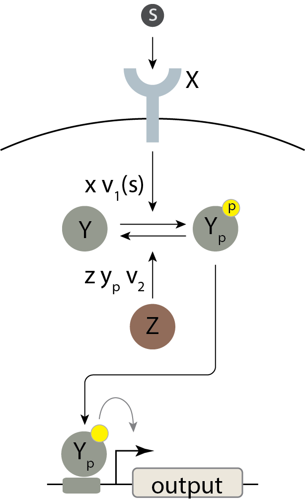
Using the analysis techniques for Michaelis-Menten kinetics that we introduced in the previous chapter, we can determine the system’s response behavior. If we assume the enzymes operate at saturation, we have

\begin{align} \frac{\mathrm{d}y_p}{\mathrm{d}t} = v_1(s)\,x \, y - v_2\,z \, y_p. \end{align}

We also have conservation of mass. Defining \(y_0\) to be the total concentration of Y, we have \(y_0 = y + y_p\). Using this expression, we have

\begin{align} \frac{\mathrm{d}y_p}{\mathrm{d}t} = v_1(s)\,x \, (y_0-y_p) - v_2\,z \, y_p. \end{align}

We can solve for the steady state concentration of phosphorylated Y, which will affect the expression of the target gene, by setting \(\mathrm{d}y_p/\mathrm{d}t = 0\) and solving. The result is

\begin{align} y_p(s) = \frac{v_1(s) x}{v_1(s)\,x + v_2 z}\,y_0 = \frac{v_1(s) x/v_2 z}{1 + v_1(s) x/v_2 z}\,y_0. \end{align}

Looking at our expression for \(y_p(s)\), we see that it takes a similar functional form to a Hill activation function of \(v_1(s)\) with \(n=1\), which can indeed be approximated by a linear function in the regime \(v_1(s)/v_2 \ll z/x\).

However, the expression for this threshold value of \(v(s_1)\), \(v_2 z/x\), includes terms for the concentrations of Z and X. Normally in a Hill function, this threshold is given by a biochemical parameter, \(k\), which represents the binding affinity of the regulator to its binding site. Such a parameter is not expected to change significantly within a given cellular environment. By contrast, in our \(y_p(s)\) expression, variations in the concentrations of Z and X could dynamically alter the location of the threshold for linearity, changing the overall shape of the response function itself! Since the target gene has no way to directly sense the concentrations of X and Z, this will significantly compromise the ability of the output to faithfully encode the concentration of the input. You can see how the response function changes as X and Z change in the interactive plot below.

# Initial parameters
x = 3
z = 0.5
v2 = 1

# x-y data for plotting
v1s = np.linspace(0, 3, 200)
yp = v1s * x / (v1s * x + v2 * z)

# Place the data in a ColumnDataSource
cds = bokeh.models.ColumnDataSource(dict(v1s=v1s, yp=yp))

# Build the plot
p = bokeh.plotting.figure(
    frame_height=150,
    frame_width=300,
    x_axis_label="v₁(s) / v₂",
    y_axis_label="steady-state yₚ / y₀",
    title="Simple Two-Component System",
    x_range=[0, 3],
    y_range=[-0.025, 1.025],
    tools="save",
)

p.line(source=cds, x="v1s", y="yp", line_width=2)

x_slider = bokeh.models.Slider(
    title="x/y₀", start=0.01, end=5, step=0.01, value=x, width=150
)
z_slider = bokeh.models.Slider(
    title="z/y₀", start=0.01, end=5, step=0.01, value=z, width=150
)


js_code = """
let yp = cds.data['yp'];
let v1s = cds.data['v1s'];
let x = x_slider.value;
let z = z_slider.value;

for (let i = 0; i < yp.length; i++) {
  yp[i] = v1s[i] * x / (v1s[i] * x + z);
}

cds.change.emit();
"""

callback = bokeh.models.CustomJS(
    args=dict(
        cds=cds,
        x_slider=x_slider,
        z_slider=z_slider,
        yaxis=p.yaxis,
    ),
    code=js_code,
)
x_slider.js_on_change("value", callback)
z_slider.js_on_change("value", callback)

layout = bokeh.layouts.row(
    p,
    bokeh.models.Spacer(width=30),
    bokeh.layouts.column(bokeh.models.Spacer(height=15), x_slider, z_slider),
)

bokeh.io.show(layout)

To overcome this obstacle, and improve the fidelity of \(y_p\)’s encoding of \(s\), we need \(y_p\) to somehow depend only on the concentation of the signaling molecule, \(s\), independent of the concentrations of X, Y, and Z. But how…?

Bifunctional kinases make two-component signaling systems robust to variation in their own components

The solution to this conundrum comes from a perplexing feature of many two-component systems: The same histidine kinase protein responsible for transferring phosphates to the response regulator also has a distinct, and nearly opposite, activity. It is not only a kinase, but also a phosphatase (a protein that catalyzes the hydrolysis of the phosphate group from the phosphorylated protein). The phosphatase activity occurs only when the histidine kinase is not itself phosphorylated.

Given its two functions, the kinase is described as bifunctional. Perversely, even as it giveth of the phosphate, it also taketh the phosphate away. This is an example of a more general concept called paradoxical regulation, in which the same component can have two opposite effects on the same target.

To see how this particular type of paradoxical regulation impacts the input-output behavior of the system, we will write down a modified model, in which the receptor X is a bifunctional kinase. First, to represent autophosphorylation, we assume that X is phosphorylated when in contact with the signaling molecules, S, by consuming a single ATP. In its phosphorylated form, it transfers the phosphate group to an unphosphorylated Y protein with a rate constant \(v_3\). This is its activating regulation. In its unphosphorylated state, it catalytically dephosphorylates Y with rate constant \(v_2\), giving it its paradoxical repressive regulation. This circuit thus consumes energy (ATP) by phosphorylating and dephosphorylating the same substrate, an example of a futile cycle.

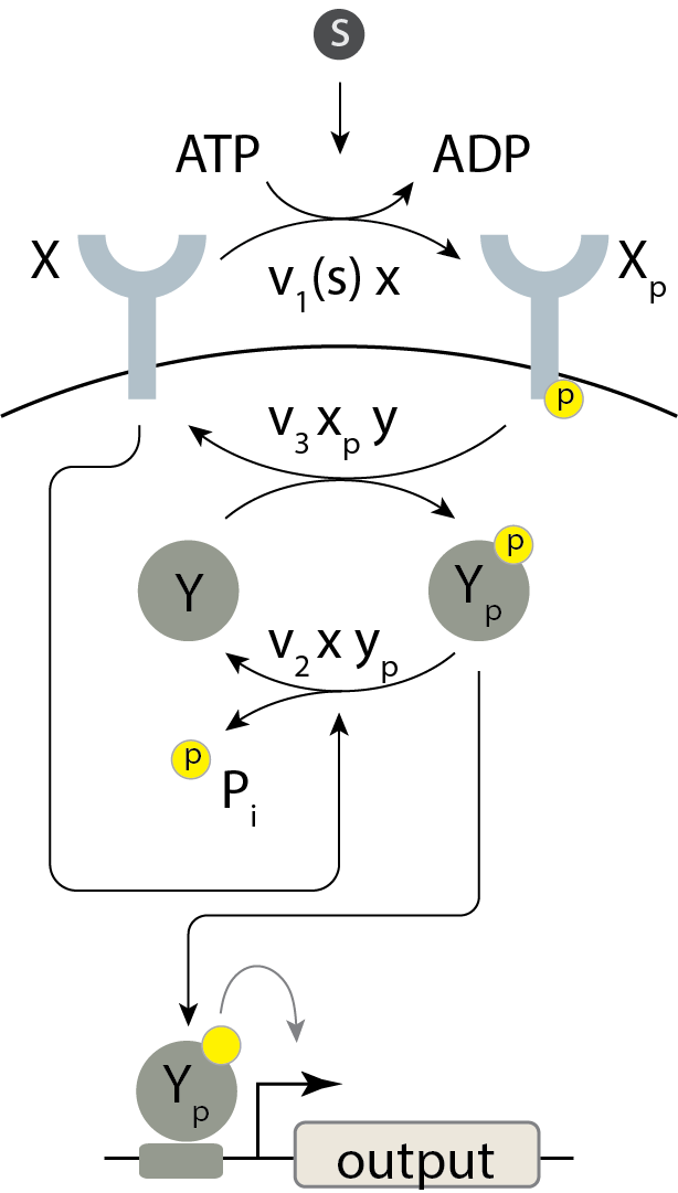
We could write out the full dynamics of this system and solve for the steady state. However, in this case there is a shortcut, introduced by Shinar et al. One can think of the multi-reaction system as a “black box.” ATP goes in, to enable kinase autophosphorylation, and ADP and inorganic phosphate come out, through the phosphatase reaction.

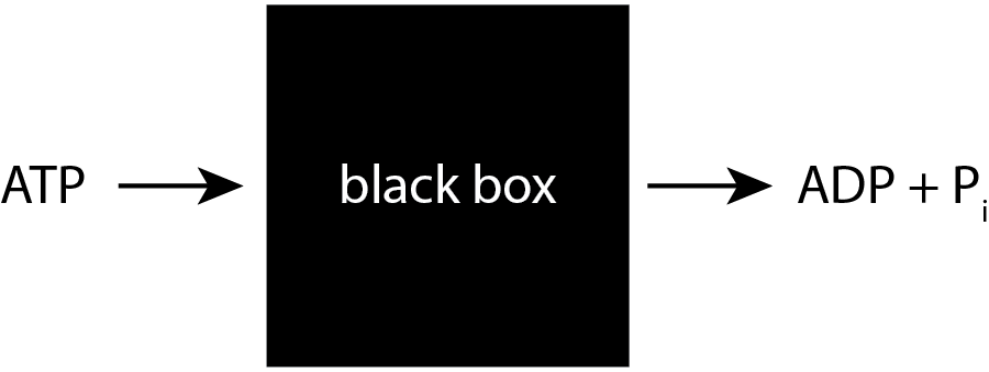
Conservation of mass dictates that the total flux of this phosphate into the system must match the total flux of Pi out of the system. The influx is \(v_1(s)\,x\) and the outflux is \(v_2\,x\,y_p\). Setting these fluxes to be equal gives

\begin{align} v_1(s)\,x = v_2\,x\,y_p, \end{align}

so that

\begin{align} y_p = \frac{v_1(s)}{v_2}. \end{align}

This is not quite complete, since we still need to respect conservation of mass of Y, so

\begin{align} y_p = \begin{cases} \frac{v_1(s)}{v_2} & y_0 \ge \frac{v_1(s)}{v_2},\\[1em] y_0 & y_0 < \frac{v_1(s)}{v_2}. \end{cases} \end{align}

Evidently, \(y_p\) depends only on \(s\), and is completely independent of the total amounts of the proteins X and Y (up to the ceiling imposed by \(y_0\)). Importantly, the activity, as quantified by the concentration of phosphorylated Y, is linear in the input \(v_1(s)\), with a slope of \(1/v_2\). Thus, this system is a perfect linear amplifier for $y_p < y_{\mathrm{tot}} $.

The following plot shows what this function looks like:

# Parameters
y0 = 1
v1s_max = 1.5

# Calculate functions
v1s_1 = np.array([0, y0])
v1s_2 = np.array([y0, v1s_max])

yp_1 = v1s_1 / y0
yp_2 = np.ones(len(v1s_2))

v1s = np.concatenate((v1s_1, v1s_2))
yp = np.concatenate((yp_1, yp_2))

# Build plot
p = bokeh.plotting.figure(
    frame_height=150,
    frame_width=300,
    x_axis_label="v₁(s) / v₂",
    y_axis_label="yₚ",
    x_range=[0, y0 * 1.5],
    tools="save"
)

p.xaxis.ticker = [0, 0.5, 1.0, 1.5]
p.xaxis.major_label_overrides = {0.5: 'y₀/2', 1: 'y₀', 1.5: '3y₀/2'}
p.yaxis.ticker = [0, 0.5, 1.0]
p.yaxis.major_label_overrides = {0.5: 'y₀/2', 1: 'y₀'}


# Plot function
p.line(v1s, yp, line_width=2)

bokeh.io.show(p)

In this model, linear amplification has the following features:

1. To achieve linearity, the cell must produce enough Y to avoid saturation over the anticipated range of input values. That is, \(y_0\) must be at least \(v_1(s_\mathrm{max})/v_2\), where \(s_\mathrm{max}\) is the maximum expected concentration of the signaling molecule.

2. It is also critical that only the dephosphorylated state of the bifunctional kinase X have phosphatase activity. If the phosphorylated state could act as a phosphatase, the inorganic phosphate balance would change, and we would lose the linear amplification feature.

3. The gain of the amplifier (the slope of the linear response) is inversely proportional to the dephosphorylation rate \(v_2\). Reducing the rate of dephosphorylation increases the gain. No pain (dephosphorylation), plenty of gain!

4. All enzymes operate at saturation, i.e. at a high ratio of substrate to enzyme. We would lose perfect linear amplification due to nonlinearities if they were not.

5. We have neglected some slow reactions. In particular, spontaneous dephosphorylation, independent of the histidine kinase, could reduce robustness to total protein levels.

Despite these restrictions and caveates, it is remarkable that a simple system can provide a function approximating perfect and robust linear amplification. This might explain the prevalence of two-component systems with bifunctional kinases.

Variant architectures

Some two-component systems have more than two components, making the term a misnomer. For example, Bacillus subtilis cells use a four-component “phosphorelay” in which histidine kinases respond to environmental insults by autophosphorylating and transferring their phosphate to a second protein, from which it is then transfered to a third, and finally a fourth protein, which is thereby activated. This terminal protein, called Spo0A, triggers sporulation, the transformation of the living cell into a dormant spore. As far as we know, it remains unclear how 4-component phosphorelays differ from the simpler 2-component architecture in their amplification properties.

An example paradoxical signaling system

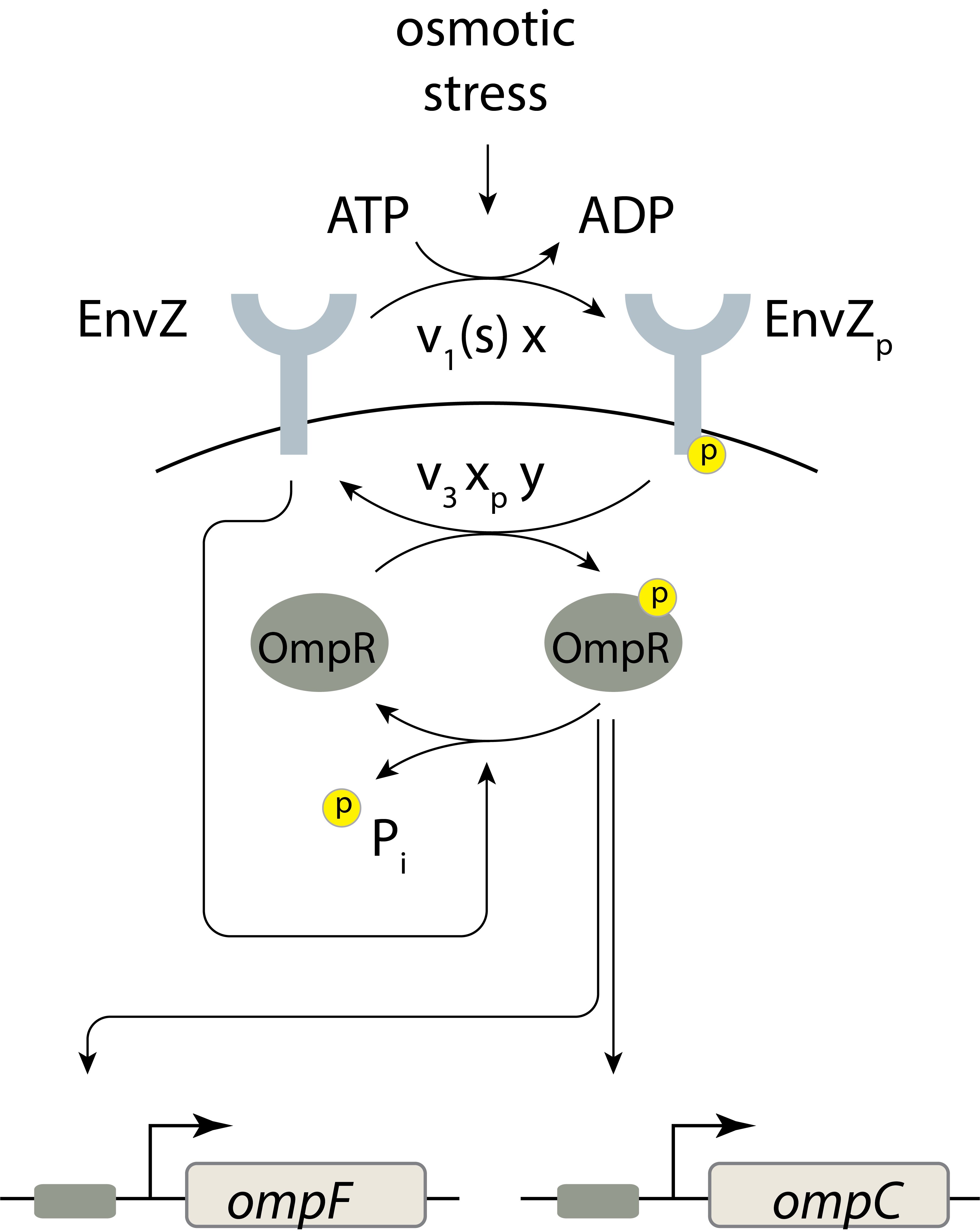
The EnvZ-OmpR system in E. coli is a classic two component system with a bifunctional kinase. EnvZ is a histidine kinase membrane protein that senses osmotic stress. It phosphorylates OmpR, which in turn regulates expression of porin genes. At high osmolarity, the cell up-regulates a large porin called OmpF, while at lower osmolarity, it predominantly expresses OmpC, which has a smaller pore.

Batchelor and Goulian (PNAS, 2003) engineered E. coli cells to express OmpR under the control of the lac promoter so they could systematically vary its expression by titrating the lactose analog IPTG. They then monitored expression of fluorescent reporter proteins expressed from OmpR’s target promoters. The compared target promoter activity at low osmolarity (in a minimal medium) and at high osmolarity (minimal medium with 15% sucrose). The result of their experiment is shown below (using data digitized from the paper).

data_low = np.array(
    [
        [-0.9731, 0.5020],
        [-0.4584, 0.9084],
        [0.0087, 0.9920],
        [0.2800, 0.8486],
        [0.5300, 0.7171],
        [0.9079, 0.7649],
        [1.0654, 0.9084],
        [1.0996, 0.9920],
        [1.1593, 1.1116],
        [1.3748, 2.2709],
    ]
)

data_high = np.array(
    [
        [-0.9787, 0.2777],
        [-0.6626, 7.6505],
        [-0.1894, 11.3891],
        [0.2365, 11.5047],
        [0.2833, 11.5021],
        [0.4325, 12.1910],
        [0.6796, 12.5956],
        [0.9735, 12.9975],
        [1.0717, 15.0837],
        [1.1288, 29.1641],
    ]
)

p = bokeh.plotting.figure(
    frame_height=250,
    frame_width=450,
    x_axis_label="fold increase in OmpR",
    y_axis_label="target promoter activity (a.u.)",
    x_axis_type="log",
    y_axis_type="log",
)
p.circle(10 ** data_low[:, 0], data_low[:, 1], legend_label="low osmolarity")
p.circle(
    10 ** data_high[:, 0],
    data_high[:, 1],
    color="orange",
    legend_label="high osmolarity",
)
p.legend.location = "center"
bokeh.io.show(p)

Astoundingly, over at least an order of magnitude the target promoter activity is robust to OmpR concentration, sensitive only to the osmolarity of the surrounding environment. This suggests that the system indeed achieves robust regulation.

Encoding ultrasensitivity: beyond cooperativity

Let’s now return back to our discussion about ultrasensitivity, above. We have seen that bifunctional two-component systems can generate almost perfect linear amplifiers through their paradoxical architecture, and thus represent ideal systems for transmitting a signal with minimal distortion.

But cells may sometimes need to respond in more of an all-or-none manner to an external stimulus. This is particularly true for yes/no decisions. Should the cell divide? Should it differentiate? Should it undergo cell death? All of these responses require a sharp, switch-like response to input signals.

When we introduced ultrasensitivty in Chapters 2 and 3 via the Hill coefficient \(n\), we pointed out that it is often achieved by cooperativity in regulatory genes. If the monomers of a transcription factor must combine to form a dimer before it can regulate its target genes, then we would expect to see a Hill coefficient up to \(n \approx 2\). Similarly, transcription factors that are only active as tetramers could yield a Hill coefficient of up to \(n \approx 4\). While this mechanism can generate ultrasensitivity, it also has some disadvantages.

For one, generating very ultrasensitive responses (\(n > 10\), for example) using only multimerization would require very large complexes. This places an architectural constraint on the structure of the proteins themselves which may compromise their other functional properties. Secondly, cooperativity is a property that is often ‘hard-wired’ into the structure of the protein itself—it is difficult to dynamically tune whether a protein complex is active only as a tetramer, only as a dimer, or only as a monomer, for example. Cells may very well face situations where they want to respond ultrasensitively to a signal, such as a hormone, in one context or cell type, but sense that same signal more linearly in a different one. In such a case, a more flexible, and dynamically tunable system for controlling ultrasensitivity would be useful.

In the next section, we will explore the eukaryotic kinase cascade circuit and show how the expression levels of its components can tune from graded to ultrasensitive responses.

The MAP kinase cascade exhibits both ultrasensitive and graded responses

The MAP (Mitogen-Activated Protein) kinase cascade is a conserved signaling system found in all eukaryotes, including yeast, plants, and mammals. Its core structure consists of a cascade of three kinases, including the eponymous MAP kinase itself (MAPK), whose active, phosphorylated form directs a downstream response. MAPK is switched into this active form through phosphorylation by the MAPK Kinase (MAPKK). MAPKK, in turn, is also active only in a phosphorylated form, which it can enter via the action of the MAPKK Kinase (MAPKKK). And MAPKKK too has active and inactive forms. As the upstream kinase in the cascade, it is phosphorylated by a variety of signals and inputs, such as growth factor receptors. Interestingly, these kinases often need to be doubly phosphorylated on two sites in order to be fully active, as indicated below by the “PP” forms.

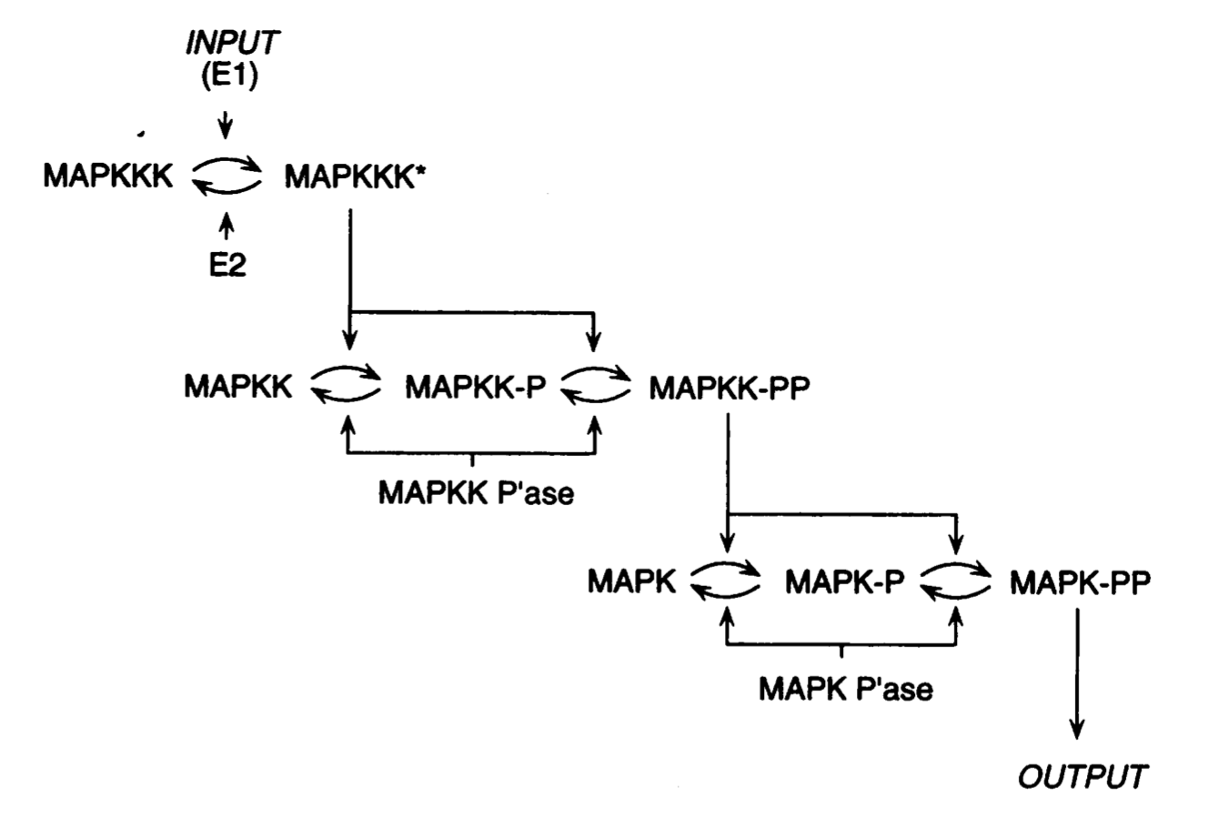
Image from Huang and Ferrell 1996, PNAS

This core pathway is duplicated in some systems, typically embedded within larger circuits, and sometimes elaborated with additional regulatory inputs. Nevertheless, the core MAPK cascade architecture is strikingly conserved and provides critical functions across a huge range of different biological systems and contexts.

Because of its central role in many critical cellular processes, the MAPK cascade has been well-studied by biologists for decades. This body of work has revealed that, in various organisms, the MAPK cascade can both exhibit an ultrasensitive response (see Huang and Ferrel 1996, PNAS) and a graded response (see Poritz et al 2007, Yeast), as well as many other interesting dynamical properties (Bhalla et al 2002, Science). In particular, James Ferrell and colleagues did pioneering early studies that sought to quantitatively understand the nature of amplification in kinase cascades.

At first glance, the structure of this system appears puzzling. Why are all these intermediate kinases necessary? Can the first kinase not just directly active the downstream response, and skip the middle men (MAPKKK and MAPKK)? Has the MAPK cascade indeed evolved to produce different behaivors in each organism and context? Or, could it be that a key conserved function of this cascade is precisely its functional plasticity, i.e. its ability to operate in various different modes in different cell contexts within each species.?

In order to address this question, one would ideally like to to take a MAPK cascade and systematically analyze its input-output response across a wide range of different regimes, varying the levels of its components. O’Shaughnessy et al. (2011, Cell) used a synthetic biology approach to do just this. They built a minimal mammalian MAPK cascade in yeast. This transplantation approach helped to insulate the core motif from the many complicating regulatory interactions it would otherwise have in its native mammalian context. Importantly, the authors designed their system so that they could quantitatively control the concentration of each of the system components. Using these “control knobs,” they investigated the response profile of the cascade across these different regimes. They then compared the observed experimental behavior with expectations from a mathematical model, which we will now explore.

We will see that the extra steps in the cascade provide ‘control knobs’ that allow it to operate it as a tunable amplifier.

A mathematical model of the MAP kinase cascade

O’Shaughnessy et al. developed a mass action ODE model based on the following reaction scheme, where the environmental signal (S) propagates down through the sequential kinases until the final MAP kinase, ERK, reaches its active form (ERKpp).

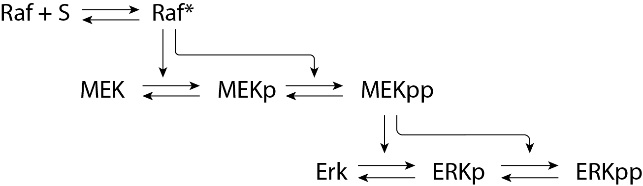
We denote the three cascade kinases as \(R\), \(M\), and \(E\), respectively, for Raf, MEK, and ERK. To represent the input, the authors assume that S binds directly to R to create an active Raf kinase, denoted \([R \cdot S]\). Each subsequent phosphorylation step is treated as a Michaelis-Menten reaction (see Chapter 6). For example, \(M + [R \cdot S] \leftrightarrow [M \cdot R \cdot S] \rightarrow M_p + [R \cdot S]\), where \(M_p\) denotes a singly phosphorylated state of MEK. \(M_p\) can similarly be phosphorylated to produce the active, doubly phosphorylated state, \(M_{pp}\).

For each step in the cascade, one needs to specify: * Whether the multiple phosphorylation sites on the target protein are phosphorylated processively, where a single encounter with the kinase causes phosphorylation of all sites, or distributively, requiring independent kinase encounters for each site. Below, we will assume distributive phosphorylation. * Whether distinct sites can be phosphorylated only in a sequential order, or in a random order. Below, we assume sequential phosphorylation. * How the phosphorylation status at each site combine to control the kinase activity of the protein. For example, whether they combine through AND, OR, or some other logic. Below, we assume AND logic. * What the concentrations and \(K_m\) values are for each reaction, and more generally whether the kinases are operating in saturated or unsaturated regimes.

Denoting concentrations using square brackets in order to make the notation for complexes clear, and introducing a set of numbered rate constants, \(k_i\) and \(k_{-i}\), for the various forward and reverse reactions, respectively, the authors obtained a formidable set of ODEs:

\begin{align} &\frac{\mathrm{d}[R]}{\mathrm{d}t} = \beta_R - \gamma [R] - k_1 [R][S] + k_{-1} [R\cdot S] \\[1em] &\frac{\mathrm{d}[R\cdot S]}{\mathrm{d}t} = - \gamma [R \cdot S] + k_1 [R][S] - k_{-1} [R\cdot S] - k_2 [M][R \cdot S] + k_{-2}[M\cdot R\cdot S] \\ &\;\;\;\;\;\;\;\;\;\;\;\;\;\;\;\;\;\; + k_3 [M\cdot R \cdot S] - k_4 [Mp][R\cdot S] + k_{-4}[Mp\cdot R\cdot S] + k_5[Mp\cdot R \cdot S] \\[1em] &\frac{\mathrm{d}[M]}{\mathrm{d}t} = \beta_M - \gamma [M] - k_2 [M][R\cdot S] + k_{-2} [M\cdot R\cdot S] \\[1em] &\frac{\mathrm{d}[M\cdot R\cdot S]}{\mathrm{d}t} = - \gamma [M\cdot R \cdot S] + k_2 [M][R\cdot S] - k_{-2}[M\cdot R\cdot S] - k_3 [M\cdot R\cdot S] \\[1em] &\frac{\mathrm{d}[Mp]}{\mathrm{d}t} = -\gamma [Mp] + k_3 [M\cdot R\cdot S] -k_4 [Mp][R\cdot S] + k_{-4}[Mp\cdot R \cdot S] \\[1em] &\frac{\mathrm{d}[Mp\cdot R\cdot S]}{\mathrm{d}t} = - \gamma [Mp\cdot R \cdot S] + k_4 [Mp][R\cdot S] - k_{-4}[Mp\cdot R\cdot S] - k_5 [Mp\cdot R \cdot S]\\[1em] &\frac{\mathrm{d}[Mpp]}{\mathrm{d}t} = -\gamma [Mpp] + k_5 [Mp\cdot R \cdot S] - k_6 [E][Mpp] + k_{-6}[E\cdot Mpp] \\ & \;\;\;\;\;\;\;\;\;\;\;\;\;\;\;\;\;\; + k_7 [E\cdot Mpp] - k_8[Ep][Mpp] + k_{-8}[Ep\cdot Mpp] + k_9 [Ep\cdot Mpp]\\[1em] &\frac{\mathrm{d}[E]}{\mathrm{d}t} = \beta_E - \gamma [E] - k_6 [E][Mpp] + k_{-6}[E\cdot Mpp] \\[1em] &\frac{\mathrm{d}[E\cdot Mpp]}{\mathrm{d}t} = -\gamma [E\cdot Mpp] + k_6 [E][Mpp] - k_{-6}[E\cdot Mpp] - k_7 [E\cdot Mpp] \\[1em] &\frac{\mathrm{d}[Ep]}{\mathrm{d}t} = -\gamma [Ep] + k_7[E\cdot Mpp] - k_8[Ep][Mpp] + k_{-8}[Ep\cdot Mpp] \\[1em] &\frac{\mathrm{d}[Ep\cdot Mpp]}{\mathrm{d}t} = -\gamma [Ep\cdot Mpp] + k_8[Ep][Mpp] - k_{-8}[Ep\cdot Mpp] - k_9 [Ep\cdot Mpp] \\[1em] &\frac{\mathrm{d}[Epp]}{\mathrm{d}t} = -\gamma [Epp] + k_9[Ep\cdot Mpp] \end{align}

Note that within the cell these cascades use scaffold proteins to group together kinases at different levels of regulation, which has major impacts on their ability to relay signals. A more complete model is necessary to fully account for these and other additional features of the pathway.

By changing the values of \(\beta_R,\beta_M,\beta_E\) for a given \(\gamma\), the authors were able to tune the values of the total concentrations of Raf, MEK, and ERK respectively. The authors then varied the MEK and ERK concentrations in their model while keeping the other parameters fixed, and measured the ultrasensitivity (Hill coefficient), threshold value (EC50), and signal strength of the final response. As you can see in the heatmaps below, the authors found that this core MAPK cascade circuit can exhibit a variety of response profiles (marked as symbols on the heatmaps) depending on the concentrations of the downstream kinases.

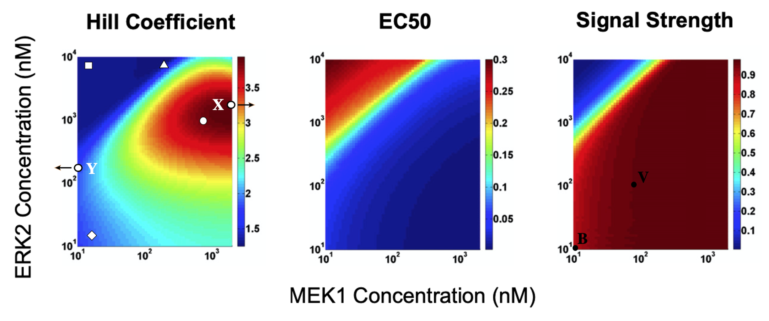
Image modified from Fig 5 of O’Shaughnessy et al 2011, Cell

To visualize the response of the concentration of doubly phosphorylated ERK to total input substrate (S) concentration. This can be calculated by integrating the above dynamical equations for various substrate concentrations and evaluating the steady states. We do this for total concentration of MEK1 and ERK that are indicated by the circle and square in the left heatmap, above. We use the same parameters as in the O’Shaughnessy et al. paper.

# Write a function to solve the ODEs for a given value of S
def MAPK_rhs(
    x,
    t,
    betaR,
    betaM,
    betaE,
    gamma,
    k1,
    k1m,
    k2,
    k2m,
    k3,
    k4,
    k4m,
    k5,
    k6,
    k6m,
    k7,
    k8,
    k8m,
    k9,
):
    R, RS, M, MRS, Mp, MpRS, Mpp, E, EMpp, Ep, EpMpp, Epp, S = x

    dR_dt = betaR - gamma * R - k1 * R * S - k1m * RS
    dRS_dt = (
        -gamma * RS
        + k1 * R * S
        - k1m * RS
        - k2 * M * RS
        + k2m * MRS
        + k3 * MRS
        - k4 * Mp * RS
        + k4m * MpRS
        + k5 * MpRS
    )
    dM_dt = betaM - gamma * M - k2 * M * RS + k2m * MRS
    dMRS_dt = -gamma * MRS + k2 * M * RS - k2m * MRS - k3 * MRS
    dMp_dt = -gamma * Mp + k3 * MRS - k4 * Mp * RS + k4m * MpRS
    dMpRS_dt = -gamma * MpRS + k4 * Mp * RS - k4m * MpRS - k5 * MpRS
    dMpp_dt = (
        -gamma * Mpp
        + k5 * MpRS
        - k6 * E * Mpp
        + k6m * EMpp
        + k7 * Mpp
        - k8 * Ep * Mpp
        + k8m * EpMpp
        + k9 * Mpp
    )
    dE_dt = betaE - gamma * E - k6 * E * Mpp + k6m * EMpp
    dEMpp_dt = -gamma * EMpp + k6 * E * Mpp - k6m * EMpp - k7 * EMpp
    dEp_dt = -gamma * Ep + k7 * EMpp - k8 * Ep * Mpp + k8m * EpMpp
    dEpMpp_dt = -gamma * EpMpp + k8 * Ep * Mpp - k8m * EpMpp - k9 * EpMpp
    dEpp_dt = -gamma * Epp + k9 * EpMpp
    dS_dt = -k1 * R * S + k1m * RS

    dx_dt = np.array(
        [
            dR_dt,
            dRS_dt,
            dM_dt,
            dMRS_dt,
            dMp_dt,
            dMpRS_dt,
            dMpp_dt,
            dE_dt,
            dEMpp_dt,
            dEp_dt,
            dEpMpp_dt,
            dEpp_dt,
            dS_dt,
        ]
    )
    return dx_dt


# Write a function that solves the ODEs for many values of S and returns the steady state value of Epp
def get_Epp_S_response_curve(
    S_vals,
    betaR,
    betaM,
    betaE,
    gamma,
    k1,
    k1m,
    k2,
    k2m,
    k3,
    k4,
    k4m,
    k5,
    k6,
    k6m,
    k7,
    k8,
    k8m,
    k9,
):
    # Number of time points we want for the solutions
    n = 10000

    # Time points we want for the solution
    t = np.linspace(0, 1e6, n)

    # Initial condition (all in uM)
    R0 = 0.010
    M0 = 0.010
    E0 = 0.010
    x0 = np.zeros(13)
    x0[0] = R0
    x0[2] = M0
    x0[7] = E0

    # Initialize vector to store Epp values
    Epp_vals = np.empty(len(S_vals))

    # Iterate over values of S
    for i, S in enumerate(S_vals):
        x0[12] = S

        # Package parameters into a tuple
        args = (
            betaR,
            betaM,
            betaE,
            gamma,
            k1,
            k1m,
            k2,
            k2m,
            k3,
            k4,
            k4m,
            k5,
            k6,
            k6m,
            k7,
            k8,
            k8m,
            k9,
        )

        # Integrate ODES
        x = scipy.integrate.odeint(MAPK_rhs, x0, t, args=args)

        # Extract Epp value and store it
        Epp_vals[i] = np.median(x[-10:, 11])

    return Epp_vals

# Parameters (units are uM and sec)
gamma = 0.001
k1 = 0.9
k1m = 0.5
k2 = 5.0
k2m = 0.5
k3 = 0.1
k4 = 5.0
k4m = 0.5
k5 = 0.1
k6 = 15.0
k6m = 0.5
k7 = 0.1
k8 = 15.0
k8m = 0.5
k9 = 0.1

# Specific concentrations for the Circle point
Rss_circ = 0.010
Mss_circ = 0.800
Ess_circ = 1.000
betaR_circ = Rss_circ * gamma
betaM_circ = Mss_circ * gamma
betaE_circ = Ess_circ * gamma

# Specific concentrations for the Square point
Rss_sq = 0.010
Mss_sq = 0.020
Ess_sq = 10.000
betaR_sq = Rss_sq * gamma
betaM_sq = Mss_sq * gamma
betaE_sq = Ess_sq * gamma


# Initialize range of S values in logspace
S_vals = np.logspace(-4, 0, 200)

# Solve
Epp_vals_circ = get_Epp_S_response_curve(
    S_vals,
    betaR_circ,
    betaM_circ,
    betaE_circ,
    gamma,
    k1,
    k1m,
    k2,
    k2m,
    k3,
    k4,
    k4m,
    k5,
    k6,
    k6m,
    k7,
    k8,
    k8m,
    k9,
)
Epp_vals_sq = get_Epp_S_response_curve(
    S_vals,
    betaR_sq,
    betaM_sq,
    betaE_sq,
    gamma,
    k1,
    k1m,
    k2,
    k2m,
    k3,
    k4,
    k4m,
    k5,
    k6,
    k6m,
    k7,
    k8,
    k8m,
    k9,
)

# Normalize outputs
Epp_vals_circ /= np.max(Epp_vals_circ)
Epp_vals_sq /= np.max(Epp_vals_sq)

# Build plot
p = bokeh.plotting.figure(
    frame_height=225,
    frame_width=300,
    x_axis_label="S (log uM)",
    y_axis_label="Epp (uM) (Normalized)",
    title=f"MAP kinase cascade, fixed parameters",
    x_axis_type='log',
    x_range=[1e-4, 1],
)

# Plot outputs
p.line(
    S_vals,
    Epp_vals_circ,
    line_width=3,
    color="#1f77b4",
    legend_label="◯ (switchlike)",
)
p.line(S_vals, Epp_vals_sq, line_width=3, color="orange", legend_label="▢ (graded)")

p.legend.location = "top_left"

# NO NEED FOR THIS
# Import in heatmap
# from bokeh.plotting import figure, show, output_file
# from bokeh.models import Div


# hm = bokeh.plotting.figure(frame_height=375, frame_width=375,)
# hm.image_url(url=["figs/MAPK_n_heatmap.png"], x=0, y=1, w=0.8, h=0.6)
# hm.xaxis.visible = False
# hm.yaxis.visible = False
# hm.xgrid.grid_line_color = None
# hm.ygrid.grid_line_color = None
# hm.outline_line_alpha = 0

# # Build layout
# MAPK_layout = bokeh.layouts.row(hm, p)

# bokeh.io.show(MAPK_layout)

bokeh.io.show(p)

We can indeed see that the minimal MAP kinase cascade is able to exhibit both graded and switchlike responses for the same choice of kinetic parameters. The only difference between the two conditions above are the values total concentrations of MEK1 and ERK2, which are tuned by changing the values of \(\beta_M\) and \(\beta_E\) with \(\gamma\) fixed. We can now see conclusively that the kinase cascade architecture enables cells to dynamically change the qualitative nature of its response, via its steepness, to the same environmental stimulus simply by changing the concentration of the kinases in the cascade.

Conclusion: phosphorylation cascades provide robust, tunable protein-level amplification

Phosphorylation appears to be a powerful mechanism for generating protein amplification systems. We have seen that these systems can provide remarkable capabilities. In a two-component system—the simplest phosphorylation cascade one can imagine—bifunctional kinases can generate linear input-output relationships, whose gain can be tuned by a single rate constant. This ability allows a pathway to convert a signal from one form to another, accurately preserving information about its level. Amazingly, this entire input-output system can be robust to the levels of its own components. Perhaps it is at least in part the combination of simplicity of design and the general usefulness of this function that accounts for the tremendous proliferation of two component systems among bacteria. E. coli has ~29 of them. B. subtilis has at least 30. And other species have even more.

Then we examined MAP kinase cascades, one of the best studied and most central circuits within the cell. We found that these systems can generate different levels of amplification and, critically, can allow the cell to modulate the sensitivity, from linear to ultrasensitive, just by modulating the concentrations of its own components. In other words, the cascade functions as a tunable amplifier, whose gain and sensitivity can differ depending on the cellular context. On the one hand, this is a powerful feature for the cell that enhances the flexibility of one of its core pathways. On the other hand, it means that just knowing that a MAP kinase cascade is involved in a process is not enough to predict how it will amplify signals. To know that, we also need to know the expression levels of kinases, and likely other related components as well.

In the future, one can imagine having a predictive model that would tell us what the gain and sensitivity of a circuit will look like based on the expression levels of its protein components—something that is increasingly available thanks to high-throughput “omics” methods. One can also consider other types of protein amplifiers. For example, within the programmed cell death pathways there are cascades of proteases that activate each other. How do such protease cascades differ in their amplification abilities compared to phosphorylation cascades?

---

References

• Batchelor, E. and Goulian, M., Robustness and the cycle of phosphorylation and dephosphorylation in a two-component regulatory system, Proc. Natl. Acad. Sci. USA, 100, 691–696, 2003. (link)

• Shinar, et al., Input–output robustness in simple bacterial signaling systems, Proc. Natl. Acad. Sci. USA, 104, 19931–19935, 2007. (link)

• Tinsley, J. N., et al., Direct detection of a single photon by humans, Nat. Commun., 7, 12172, 2016. (link)

Computing environment

%load_ext watermark
%watermark -v -p numpy,scipy,bokeh,jupyterlab

Python implementation: CPython
Python version       : 3.8.13
IPython version      : 8.3.0

numpy     : 1.21.5
scipy     : 1.7.3
bokeh     : 2.4.2
jupyterlab: 3.3.2