14. MultiFate enables expandable and controllable multistability
Design principles
Combinatorial dimerization and positive feedback generate multistability
Techniques
Phase portraits
Calculating separatrices
Key Papers
This notebook is still very much in draft form.
This draft notebook requires additional dependencies to run. In particular, you will need to install the package intersection in order to run the notebook fully. You can do this by opening a terminal window and typing
pip install intersect
and then reloading this notebook.
[1]:
# Colab setup ------------------
import os, sys, subprocess
if "google.colab" in sys.modules:
    cmd = "pip install --upgrade biocircuits intersect watermark"
    process = subprocess.Popen(cmd.split(), stdout=subprocess.PIPE, stderr=subprocess.PIPE)
    stdout, stderr = process.communicate()
    data_path = "https://biocircuits.github.io/chapters/data/"
else:
    data_path = "data/"
# ------------------------------

import numpy as np
import pandas as pd
import scipy.integrate
import scipy.optimize

import biocircuits
import biocircuits.jsplots

import bokeh.io
import bokeh.layouts
import bokeh.models
import bokeh.plotting

import colorcet

from skimage import measure

# Third-party package for finding fixed points.
# https://github.com/sukhbinder/intersection
from intersect import intersection

# Set to True to have fully interactive plots with Python;
# Set to False to use pre-built JavaScript-based plots
interactive_python_plots = False
notebook_url = "localhost:8888"

from bokeh.util.warnings import BokehUserWarning
import warnings
warnings.simplefilter(action='ignore', category=BokehUserWarning)

bokeh.io.output_notebook()
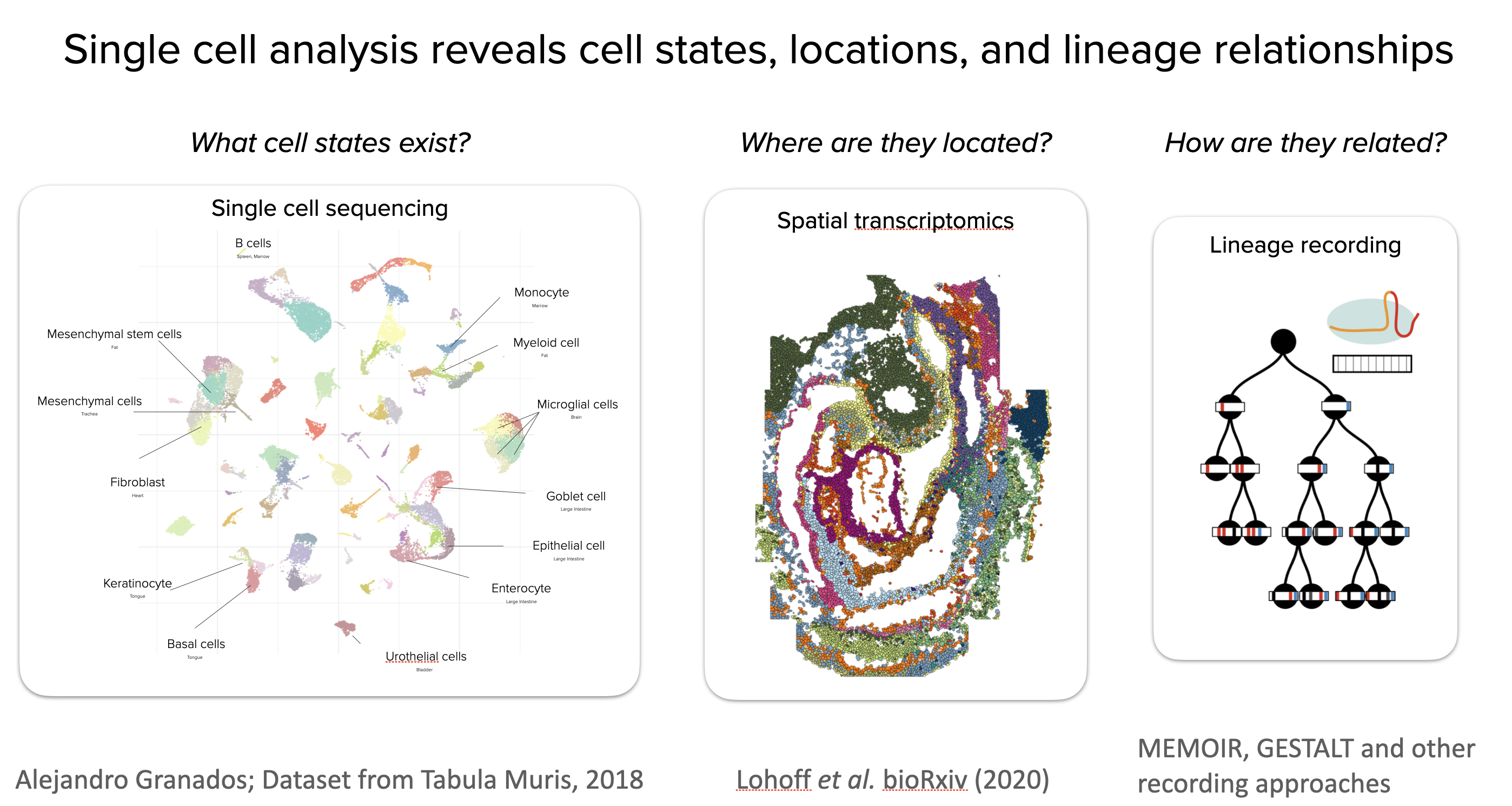
Multicellular organisms rely on a repertoire of cell states
The cells in our bodies exist in thousands of different states, differing in morphology, functional capabilities, gene expression, and other features. This multitude of cell states is generated through the astonishing process of multicellular development. As the embryo develops, cells generally commit themselves and their descendants to ever more specific cell fates: initially they decide among the germ layers—endoderm, ectoderm, and mesoderm. Later on, they will further commit to more various tissue and organ-specific cell types.
The late 2010s and early 2020s have witnessed a revolution in our understanding of cell states. Single cell “omics” techniques like single-cell RNA sequencing (scRNAseq) have revealed the molecular states of individual cells, allowing the creation of “cell atlases” of entire adult organisms. Spatial transcriptomics approaches have further shown where cells in those states are located within complex spatially organized tissues. Furthermore, emerging molecular recording techniques such as GESTALT, MEMOIR, and others are beginning to reveal the lineage relationships of individual cells, revealing how cells reached their fates. As a result, we have begun to learn what states exist, where they are located, and how they arose.
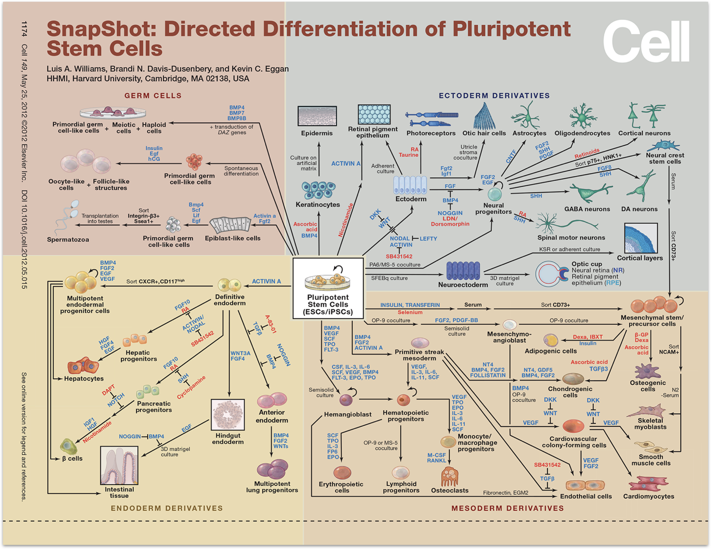
In parallel with these developments, in order to treat disease, the fields of stem cell biology and regenerative medicine have identified procedures that direct stem cells to differentiate into desired cell fates. One strategy is to recapitulate in a cell culture dish the signals that cells are likely to receive in the embryo as they differentiate into the fate of interest. This involves stimulating or inhibiting fate-controlling signaling pathways such as Notch, Wnt, Sonic hedgehog, FGF, EGF, BMP (which we covered in a previous chapter) and others, in specific sequences. A sense of the power and breadth of these approaches can be gleaned from this wall chart, published by Cell in 2012. Since then, these approaches have continued to become ever more powerful.
As a result, we now know, more than ever before, what cell types are out there and how to obtain them. Nevertheless, it has remained challenging to understand the cell fate control circuits that makes all of these incredible behaviors possible. More specifically, what architectures do those circuits use, how do they determine the repertoire of cell state that can exist in an organism? How do they control which states can differentiate to which others? And so on. In short, how do circuits specify what states can exist and how they can be controlled?
Much of our thinking has been guided by an evocative and iconic illustration from Conrad Waddington’s 1957 book, The Strategy of the Genes.
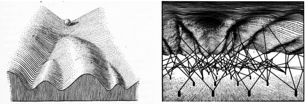
This drawing provides a wonderful intuitive metaphor for the way in which a cell, figuratively represented by a marble, might progressively commit to ever more specific cell states, by rolling deeper and deeper into alternative valleys from which is cannot easily emerge, until it eventually comes to rest in a terminally differentiated state. In the right-hand illustration, Waddington further imagined how underlying genes might control the shape of this landscape, influencing which valleys the marble is more or less likely to fall into. He represented this idea abstractly with genes (black rectangles) attached to the landscape controlling the shape of the landscape via wires (black lines). However, while these drawings are intuitively appealing and conceptually useful, they do not by themselves explain how circuits of interacting molecuels could establish and control cell fate decision-making within an organism.
One way to address this questions is by identifying the genes that specify natural cell fates and working out the ways in which they interact with one another to control cell fates. Such approaches have provided critical insights into many cell fate control systems, such as the pluripotency system that maintains embryonic stem cells in a unique ‘pluripotent’ state with the potential to differentiate into almost any cell type in the organism. A complementary approach is to try to design and build a synthetic cell fate control system “from scratch” and to see what lessons that reveals about what types of circuits are sufficient to enable such complexity. In this chapter, we will explore this latter approach.
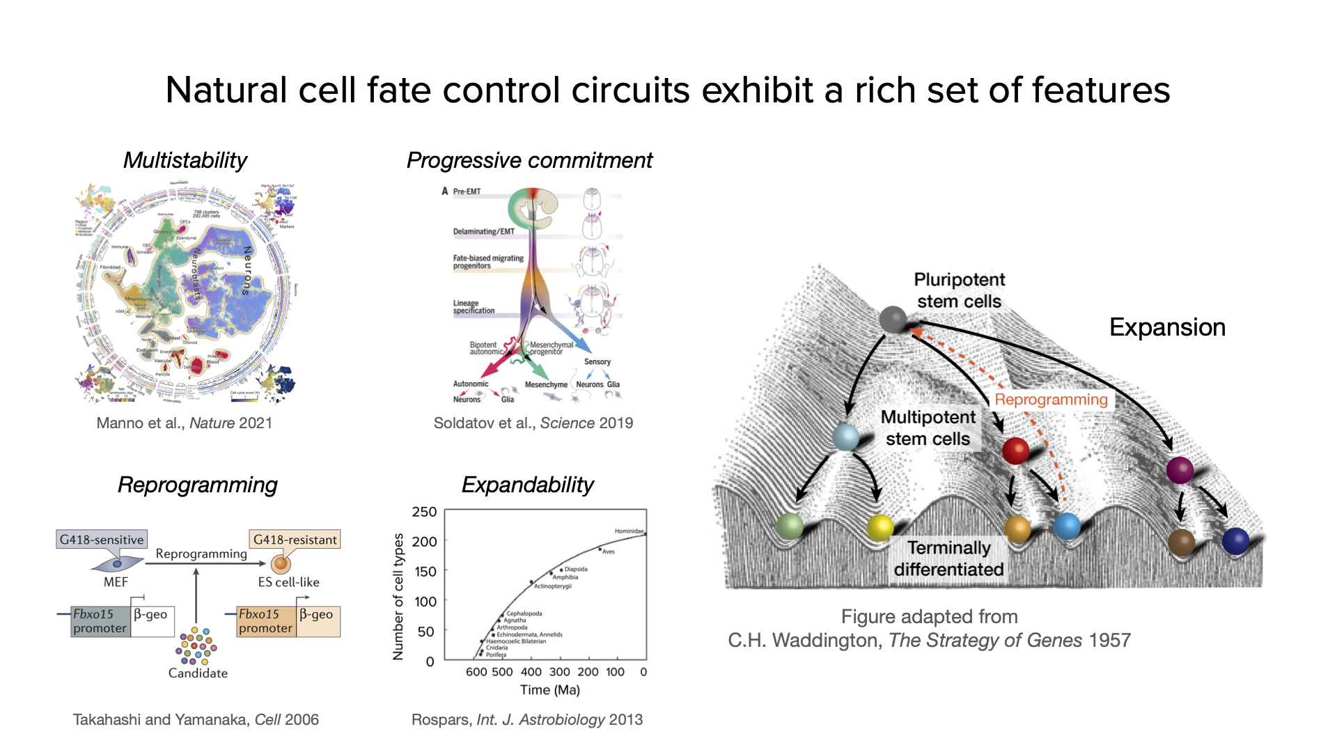
To see what we are up against in engineering a synthetic cell fate control system, consider some of the many capabilities it should, ideally, possess:
Multistability. The ideal system should be able to put cells into multiple distinct, and stable, cell states.
Progressive commitment. the system should also recapitulate the ubiquitous property of increasingly specific cell fate specification observed in so many contexts.
Reprogramming. In 2006 Takahashi and Yamanaka reported the ability to reprogram a fully differentiated cell back into an embryonic stem cell. This “rebooting” of the cell is also something a synthetic system should be able to achieve.
Expandability. During evolution, increases in organismal complexity coincided with concomitant increases in the number of different cell types in the organism. Natural cell fate control systems thus have the capacity to expand to accomodate more and more states. In the synthetic case, a similar property would enable one to expand the capacity of an engineered circuit to acheive ever more complex multicellular behaviors.
These features are illustrated here:
Can you ever imagine engineering a synthetic differentiation circuit that could rival the complexity of the complex multicellular organisms we see in nature? How would you design it?
Circuit architectures for cell differentiation
To begin to explore how these capabilities emerge from underlying circuits, we will shift from Waddington’s metaphorical diagram to a more directly applicable dynamical systems perspective.
We imagine each cell state as a stable attractor in a phase space of concentrations of transcription factors or other regulators. This representation is more general and does not require an overall “slope” down which the marble will roll.
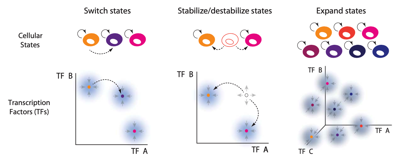
Within this general framework, the ideal circuit should:
Allow external inputs to switch cells between states.
Enable progressive commitment and reprogramming.
Expand to generate more states with additional genes.
This last feature—expandability—means that one could scale up the circuit by adding to it, e.g. incorporating additional genes, without re-engineering existing circuitry. It is important if we want the system to be able to scale to produce complex tissues or organisms with many states.
These features are diagrammed schematically here:
The first multistable circuit that may come to mind is the classic two component toggle switch, which we analyzed in Chapter 3. In principle, this circuit might be extended by incorporating many transcription factors that all repress one another. However, this would be difficult to achieve. With \(N\) transcription factors, the promoter controlling each repressor gene would have to be repressed by \(N-1\) repressors. This could become impractical given the limited available space in a promoter for effective repression. More fundamentally, however, it does not expand easily: incrememting the system from \(N\) to \(N+1\) repressors would require adding binding sites for the new repressor to all of the \(N\) existing repressors.
Before reading further, take a moment to think about what kind of architecture you might use to create a cell fate control system providing the features above.
Inspiration: natural circuits use combinatorial dimerization and positive autoregulation
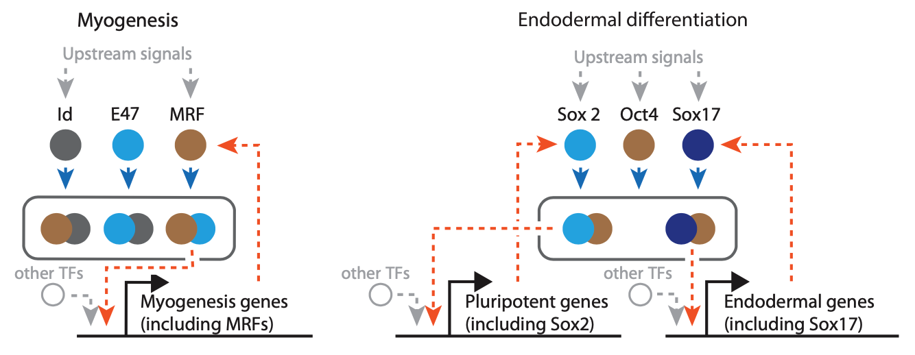
Inspiration for the design of a synthetic cell fate control system can come from looking at what is known about natural cell fate control systems. Zhu et al. (2022, Science) noticed that many natural fate control systems share two critical features:
First, they are based on sets of transcription factors that combinatorially dimerize to form many possible complexes. (This is reminescent of the combinatorial complex formation explored in the previous chapter on BMP.) Certain dimers activate downstream genes, whie others may be inactive. Formation of inactive complexes sequesters certain transcription factors, preventing them from forming alternative, active dimers with other proteins. This is analogous to the molecular titration motif we analyzed in Chapter 12.
Second, these circuits contain positive autoregulatory feedback loops, in which transcription factor dimers activate expression of one or more of their own constituents.
For example, in the circuit controlling muscle cell differentiation, the master transcription factor MyoD can dimerize with Id or E47. The MyoD-Id dimer is inactive. But te MyoD-E47 dimer transcriptionall activates many genes involved in myogenesis, including MyoD itself. Similarly, embryonic stem cells can remain in a “pluripotent” state in which they have the potential to differentiate into virtually all cell types in the embryo. The circuit that controls this state includes the key transcription factor Oct4, which can dimerize with either Sox2 or Sox17. Sox2-Oct4 and Sox17-Oct4 respectively activate expression of Sox2 and Sox17, generating autoregulation.
MultiFate: a naturally inspired synthetic cell fate control circuit
Intrigued and inspired by these architectures, Zhu et al. desigend a circuit called MultiFate, which incorporates the two themes of combinatorial dimerizaton among a set of transcription factors and positive autoregulation. We will see that the MultiFate architecture can generate multistability and the other features enough, but is simple enough to be constructed and analyzed synthetically within cells.
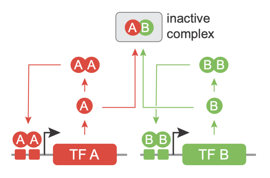
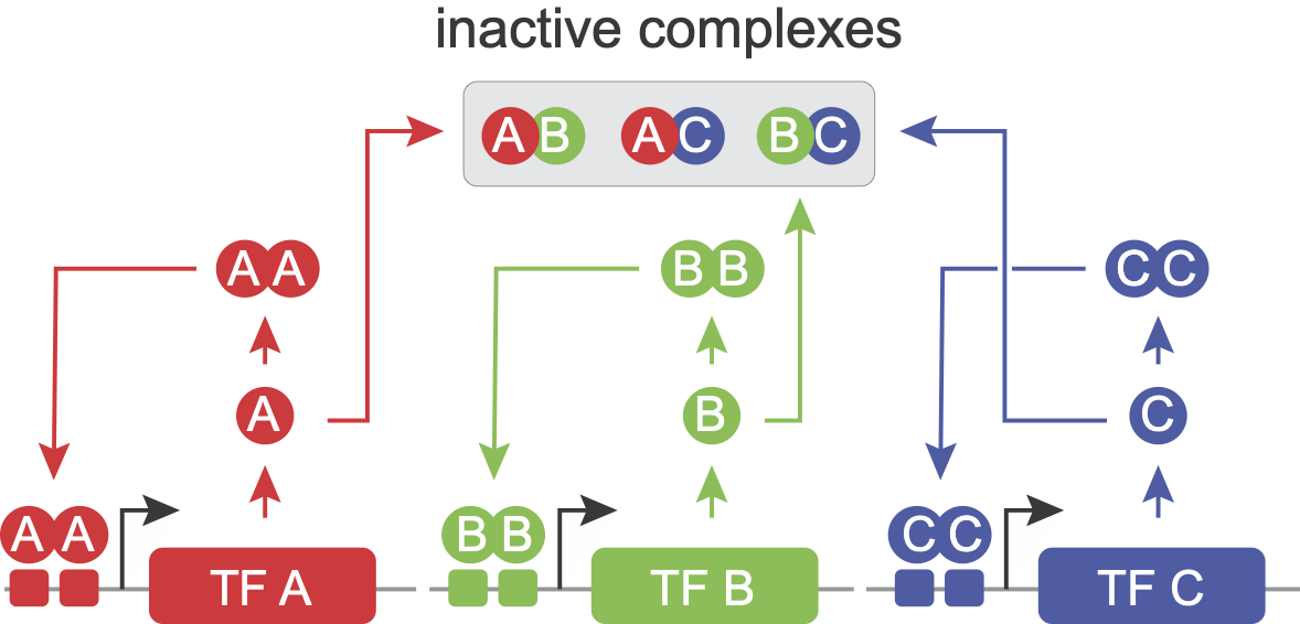
We will start by analzying a minimal version of the MultiFate architecture, termed MultiFate-2, comprising just two transcription factors, which we label A and B. A and B can each form homodimers. They can also heterodimerize with one another. The homodimers positively activate their own gene, while heterodimers are inactive. The reason that homodimers can activate their own genes, while the corresponding monomers cannot is that the DNA binding site for the dimer is effectively double the length of that of the monomer, providing approximately twice the binding energy.
The schematic drawing below explains the structure of MultiFate-2.
A two-dimensional model of MultiFate dynamics
How many states can this architecture generate? Can it be expanded? And what other dynamic properties does it possess? To find out, we will apply the approaches developed previously with additional phase plane analysis.
To begin, we will define a few variables. The A and B transcription factors can each exist either in monomeric, homodimeric, or heterodimeric form. We will represent their concentrations by the variables \([A]\) (or \([B]\)), \([A_2]\) (or \([B_2]\)), and \([AB]\), respectively.
Transcription factors can interconvert between these forms via the binding reactions:
\begin{align} & A + A \rightleftharpoons A_2 \\ & A + B \rightleftharpoons AB \\ & B + B \rightleftharpoons B_2. \end{align}
All of the binding reactions, whether they lead to homodimers or heterodimers, occur through the same type of protein-protein interaction mediated by a single engineered homodimerization motif that is incorporated in both of the synthetic transcription factors. The homodimerization reactions will therefore share a single equilibrium binding constant \(K_d\). The factor of 2 that appears in the heterodimerization reaction is a correction factor to account for the fact that the same heterodimer can form in two different ways (A+B and B+A). It prevents double-counting.
When we set these binding reactions to equilibrium, we have
\begin{align} & [A_2] = [A]^2/K_d \\ & [B_2] = [B]^2/K_d \\ & [AB] = 2[A][B]/K_d. \end{align}
We will now apply separation of timescales, making the quasi-steady-state assumption that the binding reactions are approximately at equilibrium over the timescales over which the total concentrations, \([A_{\mathrm{tot}}] = [A] + [AB] + 2[A_2]\), change due to their production and removal. We can then write down a set of ODEs that describe the slower timescale dynamics, incorporating positive autoregulation by the homodimers:
\begin{align} & \frac{\mathrm{d}[A_{\mathrm{tot}}]}{\mathrm{d}t} = \alpha + \frac{\beta [A_2]^n}{K_M^n + [A_2]^n} - \delta [A_{\mathrm{tot}}] \\ & \frac{\mathrm{d}[B_{\mathrm{tot}}]}{\mathrm{d}t} = \alpha + \frac{\beta [B_2]^n}{K_M^n + [B_2]^n} - \delta [B_{\mathrm{tot}}] \end{align}
Finally, we note that binding and unbinding reactions conserve mass:
\begin{align} & [A_{\mathrm{tot}}] = [A] + 2 [A_2] + [AB] \\ & [B_{\mathrm{tot}}] = [B] + 2 [B_2] + [AB] \end{align}
Conservation of mass reduces the model to two dimensions
These equations make a few choices and assumptions. First, we chose to use \([A_{\mathrm{tot}}]\) and \([B_{\mathrm{tot}}]\) as the dynamical variables appearing in the \(d/dt\) terms on the left hand side. This decision will simplify the analysis below, and is reasonable because it is these “total” concentrations that vary over the slower timescsales we will be interested in. Second, we represented transcriptional regulation using a leaky Hill function regulated by the homodimeric form of the transcription factor, with leak term \(\alpha\) and half-activation constant \(K_M\). The inclusion of this basal transcription is important for allowing the system to self-activate and avoiding a potential stable state in which both factors are off. (Such a state would be difficult to “read out” but could be physiologically useful in some contexts.) Finally, we assumed that removal of the two proteins occurs at the same rate regardless of whether they are in a monomeric or dimeric form, leading to the removal terms \(\delta [A_{\mathrm{tot}}]\) and \(\delta [B_{\mathrm{tot}}]\).
How many steady states can this circuit generate? And how does the answer depend on its parameters? To find out, we will solve for the steady states by setting the time derivatives to zero. Our two ODEs contain four variables: \([A_{\mathrm{tot}}], [B_{\mathrm{tot}}], [A_2], [B_2]\). To make this solvable (2 equations with 2 unknowns) we need to eliminate two of these variables. Using the equilibrium binding relations we obtained above, alongside the conservation of mass expressions, we can obtain an expression that represents \([A_2]\) and \([B_2]\) as a function of \([A_{\mathrm{tot}}]\) and \([B_{\mathrm{tot}}]\).
We accomplish this by the following procedure:
Rewrite the equilibrium binding relations so that everything is a function of the homodimer concentrations, i.e. \begin{align}&[A] = \sqrt{K_d[A_2]} \\ &[AB] = 2[A][B]/K_d = 2\sqrt{[A_2][B_2]}\end{align}
Substitute these expressions into the conservation law to obtain an equation relating the total concentrations to the homodimer concentrations only.
Rearrange the terms and solve the resulting system of equations to obtain expressions for the homodimer concentrations as a function of just the total concentrations.
Following the above process, we obtain \begin{align} & [A_2] = \frac{2 [A_{\mathrm{tot}}]^2}{K_d + 4\left([A_{\mathrm{tot}}] + [B_{\mathrm{tot}}]\right) + \sqrt{K_d^2 + 8\left([A_{\mathrm{tot}}] + [B_{\mathrm{tot}}]\right)K_d}} \\ & [B_2] = \frac{2 [B_{\mathrm{tot}}]^2}{K_d + 4\left([A_{\mathrm{tot}}] + [B_{\mathrm{tot}}]\right) + \sqrt{K_d^2 + 8\left([A_{\mathrm{tot}}] + [B_{\mathrm{tot}}]\right)K_d}}. \end{align}
If we substitute these expression back into our ODEs, then we now have a closed-form system where the rate of change of \([A_{\mathrm{tot}}]\) and \([B_{\mathrm{tot}}]\) are written as functions of only themselves.
Nondimensionalizing further simplifies the MultiFate model
Since the above expressions contain many parameters, it will be useful to nondimensionalize the system. We can make the substitutions
\begin{align} \tilde{t} &\leftarrow t\delta \\ \tilde{[A_{tot}]} &\leftarrow [A_{tot}]/K_M \\ \tilde{[B_{tot}]} &\leftarrow [B_{tot}]/K_M \\ \tilde{[A_2]} &\leftarrow [A_2]/K_M \\ \tilde{[B_2]} &\leftarrow [B_2]/K_M \\ \tilde{\alpha} &\leftarrow \alpha/(K_M \delta) \\ \tilde{\beta} &\leftarrow \beta/(K_M \delta) \\ \tilde{K_d} &\leftarrow K_d/K_M \end{align}
and then, dropping the tildes for notational convenience, arrive at a set of nondimensionalized equations:
\begin{align} \frac{\mathrm{d}[A_{tot}]}{\mathrm{d}t} &= \alpha + \frac{\beta [A_2]^n}{1 + [A_2]^n} - [A_{tot}] \\ \frac{\mathrm{d}[B_{tot}]}{\mathrm{d}t} &= \alpha + \frac{\beta [B_2]^n}{1 + [B_2]^n} - [B_{tot}] \\ [A_2] &= \frac{2[A_{tot}]^2}{K_d + 4\left( [A_{tot}] + [B_{tot}]\right) + \sqrt{K_d^2 + 8\left([A_{tot}] + [B_{tot}]\right)K_d}} \\ [B_2] &= \frac{2[B_{tot}]^2}{K_d + 4\left( [A_{tot}] + [B_{tot}]\right) + \sqrt{K_d^2 + 8\left([A_{tot}] + [B_{tot}]\right)K_d}} \end{align}
The MultiFate Phase portrait
Calculating nullclines
Plotting nullclines can be used to identify steady states and provide insight into the structure of a dynamical system. Even better, we can make the nullcline plot interactive, allowing us to see directly how different features depend on biochemical parameters. Recall from our analysis of the Toggle Switch in Chapter 3 that for a two-dimensional ODE system there will be two nullclines, one corresponding to all of the points in the plane where \(\mathrm{d}[A_{tot}]/\mathrm{d}t = 0\), and one corresponding to all of the points in the plane where \(\mathrm{d}[B_{tot}]/\mathrm{d}t = 0\). When the nullclines intersect, both ODEs are equal to zero and the system is at a fixed point.
The functional forms of the ODEs are complex, making it difficult to obtain a closed-form analytical expression for the nullclines. Instead, we will use numerical methods. Specifically, in order to find the \(\mathrm{d}[A_{tot}]/\mathrm{d}t\) nullcline we will calculate the value of \(\mathrm{d}[A_{tot}]/\mathrm{d}t\) across a grid of points in the plane, and then use the find_countours function from the scikit-measure package to find the points where
\(\mathrm{d}[A_{tot}]/\mathrm{d}t\) takes a particular value (in this case, zero). The same procedure can be used to find theh \(\mathrm{d}[B_{tot}]/\mathrm{d}t\) nullcline. This is way of doing it represents a kind of hack—its accuracy is limited—but it is convenient and can work in many situations.
The result can be seen in the interactive plot below. (Note that because this contour-finding method is not fast, the sliders on the plot are throttled so that the plot only updates when you let go of the mouse button as you move the slider.)
[2]:
class BSParams(object):
    """
    Container for parameters for homodimeric bistable circuits.
    Includes asymmetry parameters r, m, kappa, gamma.
    """
    def __init__(self, **kwargs):
        # Dimensionless parameters
        self.alpha = 0.1*2 # leakiness
        self.beta = 10*2 # Maximal production
        self.Kd = 1 # Dissociation constant of dimers
        self.n = 1.5 # Additional cooperativity of transcriptional activation
        self.r = 1 # Leakiness ratio
        self.m = 1 # A and B copy number ratio
        self.kappa = 1 # Ratio of A and B's binding affinity with DNA
        self.gamma = 1 # Ratio of stability between A and B

        # Put in params that were specified in input
        for entry in kwargs:
            setattr(self, entry, kwargs[entry])

def df_dt(y, t, p):
    """
    ODE of A and B based on parameters p.
    Includes asymmetry parameters r, m, kappa, gamma
    """
    Atot, Btot = y
    A2 = 2*Atot**2 / (p.Kd + 4*(Atot+Btot) + np.sqrt(p.Kd**2 + 8 * (Atot+Btot) * p.Kd))
    B2 = 2*Btot**2 / (p.Kd + 4*(Atot+Btot) + np.sqrt(p.Kd**2 + 8 * (Atot+Btot) * p.Kd))

    return [p.alpha + p.beta * A2**p.n / (1**p.n + A2**p.n) - Atot,
            p.alpha + p.beta * B2**p.n / (1**p.n + B2**p.n) - Btot]

def get_nullclines(params):
    """
    Calculate nullclines for Atot and Btot based on parameters.
    Includes asymmetry parameters r, m, kappa, gamma
    """
    density = 1000
    rangescale = 1.5

    Amin = params.alpha*0.01
    Amax = rangescale*params.beta
    Bmin = params.r*params.alpha*0.01
    Bmax = rangescale*params.m*params.beta

    A_vals = np.linspace(Amin, Amax, density)
    B_vals = np.linspace(Bmin, Bmax, density)

    dAdt_vals = np.zeros((len(A_vals), len(B_vals)))
    dBdt_vals = np.zeros((len(A_vals), len(B_vals)))

    AA, BB = np.meshgrid(A_vals, B_vals)

    # dummy time variable
    t = np.linspace(0,100,10)

    dAdt_vals, dBdt_vals = df_dt([AA, BB], t, params)

    Anull_inds = measure.find_contours(dAdt_vals, 0)
    Bnull_inds = measure.find_contours(dBdt_vals, 0)

    assert len(Anull_inds) == 1
    assert len(Bnull_inds) == 1

    Anull_inds = Anull_inds[0]
    Bnull_inds = Bnull_inds[0]

    A_nullcline = np.empty((len(Anull_inds), 2))
    A_nullcline[:,0] = A_vals[[int(Anull_inds[i,0]) for i in range(len(Anull_inds))]]
    A_nullcline[:,1] = Amin + (Amax-Amin)*Anull_inds[:,1]/density

    B_nullcline = np.empty((len(Bnull_inds), 2))
    B_nullcline[:,0] = Bmin + (Bmax-Bmin)*Bnull_inds[:,0]/density
    B_nullcline[:,1] = B_vals[[int(Bnull_inds[i,1]) for i in range(len(Bnull_inds))]]

    return A_nullcline, B_nullcline
[3]:
# initial plotting
params = BSParams()
params.alpha = 0.2
params.beta = 15
params.Kd = 1
params.n = 1
params.r = 1
params.m = 1
params.kappa = 1
params.gamma = 1

A_nullcline, B_nullcline = get_nullclines(params)

cdsA = bokeh.models.ColumnDataSource(dict(Anull_Avals=A_nullcline[:,0], Anull_Bvals=A_nullcline[:,1]))
cdsB = bokeh.models.ColumnDataSource(dict(Bnull_Avals=B_nullcline[:,0], Bnull_Bvals=B_nullcline[:,1]))

# Build the plot
p = bokeh.plotting.figure(
    frame_height=300,
    frame_width=300,
    x_axis_label="dimensionless A_tot",
    y_axis_label="dimensionless B_tot",
)
p.line(source=cdsA, x="Anull_Avals", y="Anull_Bvals", line_width=2, legend_label='A_tot nullcline')
p.line(source=cdsB, x="Bnull_Avals", y="Bnull_Bvals", line_width=2, color='orange', legend_label='B_tot nullcline')

alpha_slider = bokeh.models.Slider(
    title="alpha", start=0.1, end=0.5, step=0.1, value=0.2, width=150
)
beta_slider = bokeh.models.Slider(
    title="beta", start=0.5, end=17, step=0.1, value=15, width=150
)
Kd_slider = bokeh.models.Slider(
    title="Kd", start=0.5, end=10, step=0.1, value=1, width=150
)
n_slider = bokeh.models.Slider(
    title="n", start=0.5, end=3, step=0.1, value=1, width=150
)
r_slider = bokeh.models.Slider(
    title="r", start=0.1, end=10, step=0.1, value=1, width=150
)
m_slider = bokeh.models.Slider(
    title="m", start=0.1, end=10, step=0.1, value=1, width=150
)
kappa_slider = bokeh.models.Slider(
    title="kappa", start=0.1, end=10, step=0.1, value=1, width=150
)
gamma_slider = bokeh.models.Slider(
    title="gamma", start=0.1, end=10, step=0.1, value=1, width=150
)

def callback(attr, old, new):

    params = BSParams()
    params.alpha = alpha_slider.value
    params.beta = beta_slider.value
    params.Kd = Kd_slider.value
    params.n = n_slider.value
    params.r = r_slider.value
    params.m = m_slider.value
    params.kappa = kappa_slider.value
    params.gamma = gamma_slider.value

    Anull, Bnull = get_nullclines(params)
    cdsA.data["Anull_Avals"] = Anull[:,0]
    cdsA.data["Anull_Bvals"] = Anull[:,1]
    cdsB.data["Bnull_Avals"] = Bnull[:,0]
    cdsB.data["Bnull_Bvals"] = Bnull[:,1]

alpha_slider.on_change("value_throttled", callback)
beta_slider.on_change("value_throttled", callback)
Kd_slider.on_change("value_throttled", callback)
n_slider.on_change("value_throttled", callback)
r_slider.on_change("value_throttled", callback)
m_slider.on_change("value_throttled", callback)
kappa_slider.on_change("value_throttled", callback)
gamma_slider.on_change("value_throttled", callback)

layout = bokeh.layouts.row(
    p, bokeh.models.Spacer(width=30), bokeh.layouts.column(alpha_slider, beta_slider, Kd_slider, n_slider,
#                                                            r_slider, m_slider, kappa_slider, gamma_slider
                                                          )
)

def app(doc):
    doc.add_root(layout)

if interactive_python_plots:
    bokeh.io.show(app, notebook_url=notebook_url)
else:
    bokeh.io.show(p)
Determining the stability of the fixed points
With the default parameters in the plot, you can count five nullcline intersections, or fixed points. For a cell fate control system we are interested in those that are stable. To determine their stability we return to Linear Stability Analysis (see Chapter 9).
Recall that to determine stability we evaluate the Jacobian matrix of partial derivatives, \(J\), at the fixed point of interest \((x_0, y_0)\):
\begin{align} J(x_0, y_0) = \left.\begin{bmatrix}J_{0,0} & J_{0,1} \\ J_{1,0} & J_{1,1} \end{bmatrix} \right|_{(x_0, y_0)} = \left.\begin{bmatrix}\frac{\partial f(x,y)}{\partial x} & \frac{\partial f(x,y)}{\partial y} \\ \frac{\partial g(x,y)}{\partial x} & \frac{\partial g(x,y)}{\partial y} \end{bmatrix} \right|_{(x_0, y_0)} \end{align}
for \(f(x,y) = \mathrm{d}[A_{tot}]/\mathrm{d}t\) and \(g(x,y) = \mathrm{d}[B_{tot}]/\mathrm{d}t\), where we have substituted \([A_{tot}]\) and \([B_{tot}]\) with \(x\) and \(y\), respectively, for notational convenience.
In order to find the locations of these fixed points, we can once again turn to numerical approaches— in this case, we will use the intersect package developed by Sukhbinder Singh, which identifies the intersection points of two curves.
Once we find a given intersection \((x_0, y_0)\), we know it is a fixed point so we can proceed to evaluating the Jacobian matrix at that point. However, the functions \(f(x,y)\) and \(g(x,y)\) have complicated functional forms. Since we are using these derivatives in the context of an otherwise fully numerical analysis of the system, we can take advantage of a symbolic mathematical calculator to determine closed-form expressions for these derivatives:
\begin{align} &J_{0,0} = -1 - \beta \left(1 + \left(\frac{K_d + 4(x_0 + y_0) + Q}{2x_0^2}\right)^n\right)^{-2} n \left(\frac{K_d + 4(x_0 + y_0) + Q}{2x_0^2}\right)^{n-1} \left(\frac{x_0 \left(4 + \frac{4K_d}{Q}\right) - 2(K_d + 4(x_0 + y_0) + Q)}{2x_0^3} \right) \\ &J_{0,1} = - \beta \left(1 + \left(\frac{K_d + 4(x_0 + y_0) + Q}{2x_0^2}\right)^n\right)^{-2} n \left(\frac{K_d + 4(x_0 + y_0) + Q}{2x_0^2}\right)^{n-1}\left(\frac{4 + \frac{4K_d}{Q} }{2x_0^2} \right) \\ &J_{1,0} = - \beta \left(1 + \left( \frac{K_d + 4(x_0 + y_0) + Q}{2y_0^2}\right)^n\right)^{-2}n \left(\frac{K_d + 4(x_0 + y_0) + Q}{2y_0^2}\right)^{n-1}\left(\frac{4 + \frac{4K_d}{Q} }{2y_0^2} \right) \\ &J_{1,1} = -1 - \beta \left(1 + \left( \frac{K_d + 4(x_0 + y_0) + Q}{2y_0^2}\right)^n\right)^{-2}n \left(\frac{K_d + 4(x_0 + y_0) + Q}{2y_0^2}\right)^{n-1} \left( \frac{y_0 \left(4 + \frac{4K_d}{Q}\right) -2 (K_d + 4(x_0 + y_0) + Q)}{2y_0^3} \right), \end{align}
where
\begin{align} Q \equiv \sqrt{K_d^2 + 8(x_0 + y_0) + K_d}. \end{align}
Let’s now overlay an indicator of fixed point stability over the nullcline plots that we made.
[4]:
# Code to calcaulte the jacobian symbolically each time to confirm
# the above equations are correct

# def symbolic_jacobian(v_str, f_list):
#     varss = sym.symbols(v_str)
#     f = sym.sympify(f_list)
#     J = sym.zeros(len(f),len(varss))
#     for i, fi in enumerate(f):
#         for j, s in enumerate(varss):
#             J[i,j] = sym.diff(fi, s)
#     return J

# def get_jacobian_func(p):
#     v_str = 'Atot Btot'

#     A2 = f'(2*Atot**2 / ({p.Kd} + 4*(Atot+Btot) + sqrt({p.Kd}**2 + 8 * (Atot+Btot) * {p.Kd})))'
#     B2 = f'(2*Btot**2 / ({p.Kd} + 4*(Atot+Btot) + sqrt({p.Kd}**2 + 8 * (Atot+Btot) * {p.Kd})))'
#     f_list = [f'{p.alpha} + {p.beta}*{A2}**{p.n} / (1**{p.n} + {A2}**{p.n}) - Atot',
#              f'{p.alpha} + {p.beta}*{B2}**{p.n} / (1**{p.n} + {B2}**{p.n}) - Btot']

#     J = symbolic_jacobian(v_str, f_list)

#     return lambdify(sym.symbols(v_str), J, modules='numpy')

# def stability(x0, y0, jacobian_func):
#     jmat = jacobian_func(x0, y0)
#     eig = np.linalg.eigvals(jmat)
#     print(eig)
#     return (np.real(eig)<0).all()

# def get_fixed_points(Anull, Bnull, params):
#     # get jacobian
#     jacobian_func = get_jacobian_func(params)

#     # find fixed points
#     x, y = intersection(Anull[:,0], Anull[:,1], Bnull[:,0], Bnull[:,1])
#     stable_fp = np.empty((0,2))
#     unstable_fp = np.empty((0,2))
#     # for each fixed point, use the surrounding 4 points to determine the stability
#     for i in range(len(x)):
#         print(x[i], y[i])
#         if stability(x[i], y[i], jacobian_func)==1:
#             stable_fp = np.vstack([stable_fp, [x[i],y[i]]])
#             print('stable exissted')
#         else:
#             print('unstable existed')
#             unstable_fp = np.vstack([unstable_fp, [x[i],y[i]]])

#     return stable_fp, unstable_fp

####################
# Using the Jacobian function Ron calculated

def jacobian(x0, y0, p):
    # Calculate the jacobian matrix
    # Fixed point = (x0, y0)
    # p = parameters
    jmat = np.zeros([2,2])
    sqtemp = np.sqrt(p.Kd**2 + 8 * (x0 + y0) * p.Kd)

    jmat[0,0] = - 1 - p.beta * (1 + ((p.Kd + 4 * (x0 + y0) + sqtemp) / (2 * x0**2))**p.n)**(-2) * p.n * ((p.Kd + 4 * (x0 + y0) + sqtemp) / (2 * x0**2))**(p.n-1) * (x0 * (4 + 4 * p.Kd / sqtemp) - 2 * (p.Kd + 4 * (x0 + y0) + sqtemp)) / (2 * x0**3)
    jmat[0,1] = - p.beta * (1 + ((p.Kd + 4 * (x0 + y0) + sqtemp) / (2 * x0**2))**p.n)**(-2) * p.n * ((p.Kd + 4 * (x0 + y0) + sqtemp) / (2 * x0**2))**(p.n-1) * (4 + 4 * p.Kd / sqtemp) / (2 * x0**2)
    jmat[1,0] = - p.m * p.beta * (1 + (p.kappa * (p.Kd + 4 * (x0 + y0) + sqtemp) / (2 * y0**2))**p.n)**(-2) * p.n * (p.kappa * (p.Kd + 4 * (x0 + y0) + sqtemp) / (2 * y0**2))**(p.n-1) * p.kappa * (4 + 4 * p.Kd / sqtemp) / (2 * y0**2)
    jmat[1,1] = - p.gamma - p.m * p.beta * (1 + (p.kappa * (p.Kd + 4 * (x0 + y0) + sqtemp) / (2 * y0**2))**p.n)**(-2) * p.n * (p.kappa * (p.Kd + 4 * (x0 + y0) + sqtemp) / (2 * y0**2))**(p.n-1) * (y0 * p.kappa * (4 + 4 * p.Kd / sqtemp) - 2 * p.kappa * (p.Kd + 4 * (x0 + y0) + sqtemp)) / (2 * y0**3)

    return jmat

def stability(x0, y0, p):
    """
    Returns True if stable
    """
    # x0, y0 = fixed point coord
    # Calculate the stability of fixed point based on eigenvalue of jacobian matrix
    jmat = jacobian(x0, y0, p)
    eig = np.linalg.eigvals(jmat)
    return (np.real(eig)<0).all()

def get_fixed_points(Anull, Bnull, params):

    # find fixed points
    x, y = intersection(Anull[:,0], Anull[:,1], Bnull[:,0], Bnull[:,1])
    stable_fp = np.empty((0,2))
    unstable_fp = np.empty((0,2))
    # for each fixed point, use the surrounding 4 points to determine the stability
    for i in range(len(x)):
        if stability(x[i], y[i], params)==1:
            stable_fp = np.vstack([stable_fp, [x[i],y[i]]])
        else:
            unstable_fp = np.vstack([unstable_fp, [x[i],y[i]]])

    return stable_fp, unstable_fp
[5]:
# initial plotting
params = BSParams()
params.alpha = 0.2
params.beta = 15
params.Kd = 1
params.n = 1
params.r = 1
params.m = 1
params.kappa = 1
params.gamma = 1

A_nullcline, B_nullcline = get_nullclines(params)
stable_fps, unstable_fps = get_fixed_points(A_nullcline, B_nullcline, params)

cdsA = bokeh.models.ColumnDataSource(dict(Anull_Avals=A_nullcline[:,0], Anull_Bvals=A_nullcline[:,1]))
cdsB = bokeh.models.ColumnDataSource(dict(Bnull_Avals=B_nullcline[:,0], Bnull_Bvals=B_nullcline[:,1]))
cds_stable_fps = bokeh.models.ColumnDataSource(dict(x=stable_fps[:,0], y=stable_fps[:,1]))
cds_unstable_fps = bokeh.models.ColumnDataSource(dict(x=unstable_fps[:,0], y=unstable_fps[:,1]))

# Build the plot
p = bokeh.plotting.figure(
    frame_height=300,
    frame_width=300,
    x_axis_label="dimensionless A_tot",
    y_axis_label="dimensionless B_tot",
)
p.line(source=cdsA, x="Anull_Avals", y="Anull_Bvals", line_width=2, legend_label='A_tot nullcline')
p.line(source=cdsB, x="Bnull_Avals", y="Bnull_Bvals", line_width=2, color='orange', legend_label='B_tot nullcline')
p.scatter(
    source=cds_stable_fps,
    x="x",
    y="y",
    color="black",
    size=10,
    line_width=1
)
p.scatter(
    source=cds_unstable_fps,
    x="x",
    y="y",
    color="white",
    line_color="black",
    size=10,
    line_width=1
)

alpha_slider = bokeh.models.Slider(
    title="alpha", start=0.1, end=0.6, step=0.1, value=0.2, width=150
)
beta_slider = bokeh.models.Slider(
    title="beta", start=0.5, end=17, step=0.1, value=15, width=150
)
Kd_slider = bokeh.models.Slider(
    title="Kd", start=0.5, end=10, step=0.1, value=1, width=150
)
n_slider = bokeh.models.Slider(
    title="n", start=0.5, end=3, step=0.1, value=1, width=150
)
r_slider = bokeh.models.Slider(
    title="r", start=0.1, end=10, step=0.1, value=1, width=150
)
m_slider = bokeh.models.Slider(
    title="m", start=0.1, end=10, step=0.1, value=1, width=150
)
kappa_slider = bokeh.models.Slider(
    title="kappa", start=0.1, end=10, step=0.1, value=1, width=150
)
gamma_slider = bokeh.models.Slider(
    title="gamma", start=0.1, end=10, step=0.1, value=1, width=150
)

def callback(attr, old, new):

    params = BSParams()
    params.alpha = alpha_slider.value
    params.beta = beta_slider.value
    params.Kd = Kd_slider.value
    params.n = n_slider.value
    params.r = r_slider.value
    params.m = m_slider.value
    params.kappa = kappa_slider.value
    params.gamma = gamma_slider.value

    Anull, Bnull = get_nullclines(params)
    cdsA.data["Anull_Avals"] = Anull[:,0]
    cdsA.data["Anull_Bvals"] = Anull[:,1]
    cdsB.data["Bnull_Avals"] = Bnull[:,0]
    cdsB.data["Bnull_Bvals"] = Bnull[:,1]

    stable_fps, unstable_fps = get_fixed_points(Anull, Bnull, params)
    cds_stable_fps.data["x"] = stable_fps[:,0]
    cds_stable_fps.data["y"] = stable_fps[:,1]
    cds_unstable_fps.data["x"] = unstable_fps[:,0]
    cds_unstable_fps.data["y"] = unstable_fps[:,1]

alpha_slider.on_change("value_throttled", callback)
beta_slider.on_change("value_throttled", callback)
Kd_slider.on_change("value_throttled", callback)
n_slider.on_change("value_throttled", callback)
r_slider.on_change("value_throttled", callback)
m_slider.on_change("value_throttled", callback)
kappa_slider.on_change("value_throttled", callback)
gamma_slider.on_change("value_throttled", callback)

layout = bokeh.layouts.row(
    p, bokeh.models.Spacer(width=30), bokeh.layouts.column(alpha_slider, beta_slider, Kd_slider, n_slider,
#                                                            r_slider, m_slider, kappa_slider, gamma_slider
                                                          )
)

def app(doc):
    doc.add_root(layout)

if interactive_python_plots:
    bokeh.io.show(app, notebook_url=notebook_url)
else:
    bokeh.io.show(p)
Plotting a flow field
To investigate the behavior near the fixed points, and indeed away from them as well, we can plot the phase portrait. A phase portrait is a plot displaying possible trajectories of a dynamical system in phase space, in this case on the \(A_\mathrm{tot}\)-\(B_\mathrm{tot}\) plane. Let’s generate a phase portrait using the biocircuits package (with the nullclines overlaid).
The biocircuits.phase_portrait() function requires explicit functions for \(\mathrm{d}[A_{tot}]/\mathrm{d}t\) and \(\mathrm{d}[B_{tot}]/\mathrm{d}t\).
[6]:
def dAtot_dt(Atot, Btot, alpha, beta, n, Kd):
    A2 = (
        2
        * Atot ** 2
        / (Kd + 4 * (Atot + Btot) + np.sqrt(Kd ** 2 + 8 * (Atot + Btot) * Kd))
    )
    return alpha + beta * A2 ** n / (1 ** n + A2 ** n) - Atot


def dBtot_dt(Atot, Btot, alpha, beta, n, Kd):
    B2 = (
        2
        * Btot ** 2
        / (Kd + 4 * (Atot + Btot) + np.sqrt(Kd ** 2 + 8 * (Atot + Btot) * Kd))
    )
    return alpha + beta * B2 ** n / (1 ** n + B2 ** n) - Btot
Next, we will build a plot with the fixed points and nullclines, as before.
[7]:
# initial plotting
alpha = 0.2
beta = 15
Kd = 1
n = 1
r = 1
m = 1
kappa = 1
gamma = 1

density = 1000
rangescale = 1.5

Amin = params.alpha*0.01
Amax = rangescale*params.beta
Bmin = params.r*params.alpha*0.01
Bmax = rangescale*params.m*params.beta

params = BSParams()
params.alpha = alpha
params.beta = beta
params.Kd = Kd
params.n = n
params.r = r
params.m = m
params.kappa = kappa
params.gamma = gamma

A_nullcline, B_nullcline = get_nullclines(params)
stable_fps, unstable_fps = get_fixed_points(A_nullcline, B_nullcline, params)

cdsA = bokeh.models.ColumnDataSource(dict(Anull_Avals=A_nullcline[:,0], Anull_Bvals=A_nullcline[:,1]))
cdsB = bokeh.models.ColumnDataSource(dict(Bnull_Avals=B_nullcline[:,0], Bnull_Bvals=B_nullcline[:,1]))
cds_stable_fps = bokeh.models.ColumnDataSource(dict(x=stable_fps[:,0], y=stable_fps[:,1]))
cds_unstable_fps = bokeh.models.ColumnDataSource(dict(x=unstable_fps[:,0], y=unstable_fps[:,1]))

p = bokeh.plotting.figure(
    frame_height=300,
    frame_width=300,
    x_axis_label="dimensionless A_tot",
    y_axis_label="dimensionless B_tot",
)

p.line(source=cdsA, x="Anull_Avals", y="Anull_Bvals", line_width=2, legend_label='A_tot nullcline')
p.line(source=cdsB, x="Bnull_Avals", y="Bnull_Bvals", line_width=2, color='orange', legend_label='B_tot nullcline')
p.scatter(
    source=cds_stable_fps,
    x="x",
    y="y",
    color="black",
    size=10,
    line_width=1
)
p.scatter(
    source=cds_unstable_fps,
    x="x",
    y="y",
    color="white",
    line_color="black",
    size=10,
    line_width=1
);
Finally, we overlay the phase portrait.
[8]:
p = biocircuits.phase_portrait(
    dAtot_dt,
    dBtot_dt,
    [Amin, Amax],
    [Bmin, Bmax],
    (alpha, beta, n, Kd),
    (alpha, beta, n, Kd),
    x_axis_label="dimensionless A_tot",
    y_axis_label="dimensionless B_tot",
    color="gray",
    p=p,
)

bokeh.io.show(p)
Plotting separatrices
Notice how two trajectories can start very close to each other yet diverge and end up at different stable fixed points. The set of all starting points that eventually land on a given attractor (stable fixed point) is known as its basin of attraction. The boundary between two basins of attraction is called a separatrix.
We can calculaute the separatrices by making use of the fact that a separatrix is the one-dimensional stable manifold of a particular saddle fixed point— while trajectories on either side of a separatrix will converge to a stable fixed point, trajectories that start exactly on a separatrix will converge to a saddle point.
Recall from our exploration of Linear Stability Analysis in Chapter 9 that a saddle fixed point has one stable eigendirection and one unstable eigendirection. Near the fixed point, one eigenvector, \(\boldsymbol{v}\), and its inverse \(-\boldsymbol{v}\), point outwards from the fixed point. This eigenvector is parallel to the separatrix close to the fixed point. However, moving away from the fixed point, the eigenvector and the separatrix will begin to diverge. In order to follow the separatrix, therefore, we must start at the fixed point, take a very small stepp along the \(\boldsymbol{v}\) direction, and then follow the ODEs themselves by integrating backwards in time to find all of the trajectories that would eventually converge to the fixed point. We can then repeat this procedure in the \(-\boldsymbol{v}\) direction to find the other arm of the separatrix.
We demonstrate this procedure below.
[9]:
def df_dt_tuple(concs, t, alpha, beta, Kd, n, r, m, kappa, gamma):
    Atot, Btot = concs
    A2 = 2*Atot**2 / (Kd + 4*(Atot+Btot) + np.sqrt(Kd**2 + 8 * (Atot+Btot) * Kd))
    B2 = 2*Btot**2 / (Kd + 4*(Atot+Btot) + np.sqrt(Kd**2 + 8 * (Atot+Btot) * Kd))

    return [-1 * (alpha + beta * A2**n / (1**n + A2**n) - Atot),
            -1 * (alpha + beta * B2**n / (1**n + B2**n) - Btot)]

def plot_separatrix(
    x0,
    y0,
    A_range,
    B_range,
    params,
    p,
    t_max=100,
    eps=1e-6,
    color="#d95f02",
    line_width=2,
):
    """
    Plot separatrix on phase portrait.
    Takes bokeh plot p as an input and returns p with
    separatrix plot overlaid.
    """
    # Negative time function to integrate to compute separatrix
    def rhs(concs, t):
        # Unpack variables
        Atot, Btot = concs

        # return df_dt_tuple(concs, t, alpha, beta, Kd, n, r, m, kappa, gamma)

        # Stop integrating if we get the edge of where we want to integrate
        if A_range[0] < Atot < A_range[1] and B_range[0] < Btot < B_range[1]:
            return df_dt_tuple(concs, t, alpha, beta, Kd, n, r, m, kappa, gamma)
        else:
            return np.array([0, 0])

    # Compute eigenvalues and eigenvectors
    evals, evecs = np.linalg.eig(jacobian(x0, y0, params))

    # Get eigenvector corresponding to attraction
    evec = evecs[:, evals < 0].flatten()

    # Parameters for building separatrix
    t = np.linspace(0, t_max, 400)

    # Put parameters in a tuple
    args = (params.alpha, params.beta, params.Kd, params.n, params.r, params.m, params.kappa, params.gamma)
    alpha = params.alpha
    beta = params.beta
    Kd = params.Kd
    n = params.n
    r = params.r
    m = params.m
    kappa = params.kappa
    gamma = params.gamma

    # Build upper right branch of separatrix
    c0 = np.array([x0, y0]) + eps * evec
    x_upper = scipy.integrate.odeint(rhs, c0, t)

    # Build lower left branch of separatrix
    c0 = np.array([x0, y0]) - eps * evec
    x_lower = scipy.integrate.odeint(rhs, c0, t)

    # Concatenate, reversing lower so points are sequential
    sep_x = np.concatenate((x_lower[::-1, 0], x_upper[:, 0]))
    sep_y = np.concatenate((x_lower[::-1, 1], x_upper[:, 1]))

    # Plot
    p.line(sep_x, sep_y, color=color, line_width=line_width,legend_label="seperatrix")

    return p
[10]:
params = BSParams()
params.alpha = 0.2
params.beta = 15
params.Kd = 1
params.n = 1
params.r = 1
params.m = 1
params.kappa = 1
params.gamma = 1

Amin = params.alpha*0.01
Amax = rangescale*params.beta
Bmin = params.r*params.alpha*0.01
Bmax = rangescale*params.m*params.beta

A_nullcline, B_nullcline = get_nullclines(params)
stable_fps, unstable_fps = get_fixed_points(A_nullcline, B_nullcline, params)

cdsA = bokeh.models.ColumnDataSource(dict(Anull_Avals=A_nullcline[:,0], Anull_Bvals=A_nullcline[:,1]))
cdsB = bokeh.models.ColumnDataSource(dict(Bnull_Avals=B_nullcline[:,0], Bnull_Bvals=B_nullcline[:,1]))
cds_stable_fps = bokeh.models.ColumnDataSource(dict(x=stable_fps[:,0], y=stable_fps[:,1]))
cds_unstable_fps = bokeh.models.ColumnDataSource(dict(x=unstable_fps[:,0], y=unstable_fps[:,1]))

# Build the plot
p = biocircuits.phase_portrait(
    dAtot_dt,
    dBtot_dt,
    [Amin, Amax],
    [Bmin, Bmax],
    (alpha, beta, n, Kd),
    (alpha, beta, n, Kd),
    x_axis_label="dimensionless A_tot",
    y_axis_label="dimensionless B_tot",
    color="gray",
    plot_width=450,
)
p.line(source=cdsA, x="Anull_Avals", y="Anull_Bvals", line_width=2, legend_label='A_tot nullcline')
p.line(source=cdsB, x="Bnull_Avals", y="Bnull_Bvals", line_width=2, color='orange', legend_label='B_tot nullcline')
p.scatter(
    source=cds_stable_fps,
    x="x",
    y="y",
    color="black",
    size=10,
    line_width=1
)
p.scatter(
    source=cds_unstable_fps,
    x="x",
    y="y",
    color="white",
    line_color="black",
    size=10,
    line_width=1
)

# Calculate separatrices
for ufp in unstable_fps:
    p = plot_separatrix(ufp[0], ufp[1], [Amin, Amax],[Bmin, Bmax], params, p, eps=1e-1)

bokeh.io.show(p)
The separatrices mark the boundaries between the basins of attraction, as expected. You can see how trajectories that start on different sides of the separatrix approach different stable fixed points. Using this approach, it is possible to plot the MultiFate-2 phase portrait in a range of different parameter regimes. By doing so, one can see that this simple circuit can produce a wide array of different stability behaviors, from monostability to quadrastability:
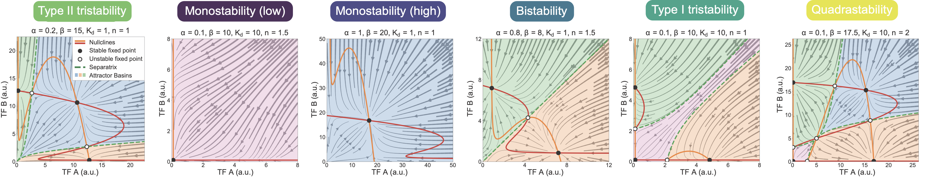
These are just the symmetric systems. Allowing asymmetric regimes, in which A and B can take on different production rates or other parameters, generates an even larger space of dynamical behaviors.
Taken together, this analysis shows that MultiFate should be able to produce a variety of different types of multistability.
Building MultiFate
Will MultiFate indeed generate multistability in cells? And, could it provide some of the key capabilities expected of an ideal cell differentiation circuit, such as multistability, state-switching, control of state stability, and expandability? To find out, Zhu et al. constructed an experimental implementation of the MultiFate-2 circuit.
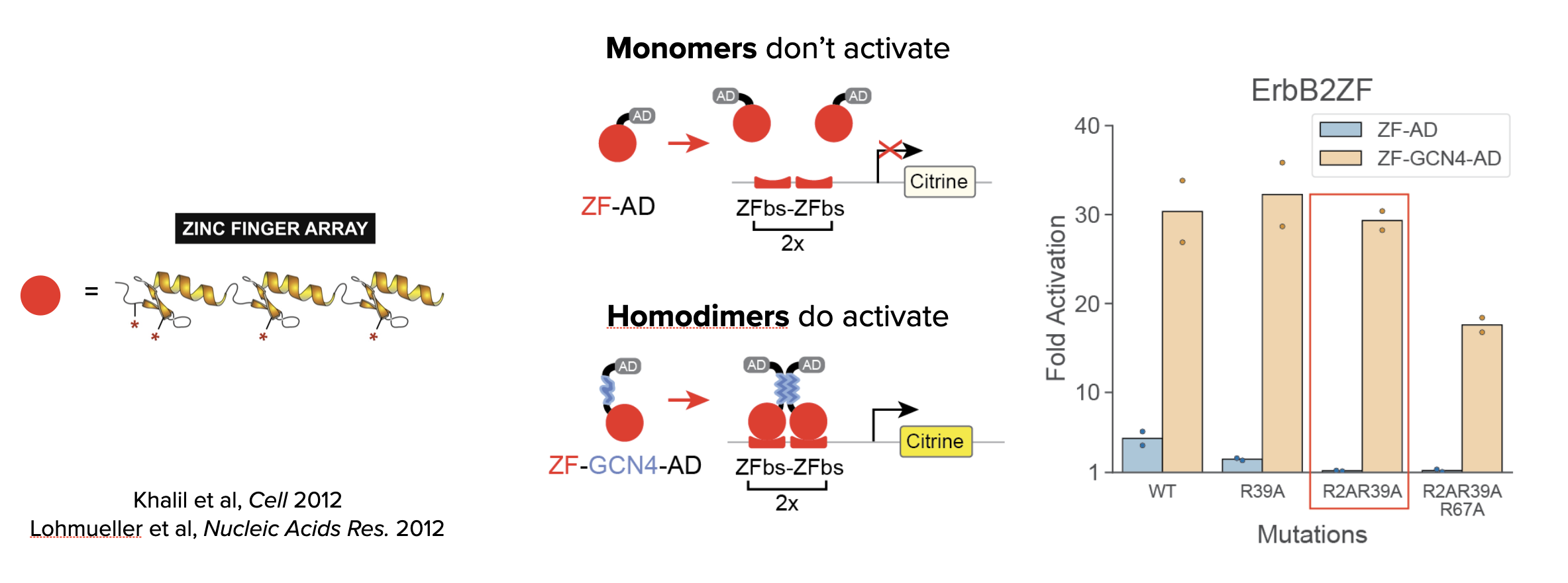
The key components required to build MultiFate are transcription factors that activate only as homodimers and inhibit each other through heterodimerization. Zinc finger DNA-binding proteins (below, left) provided an ideal type of engineerable DNA binding protein. They are comprised of modular domains (fingers) that bind to specific 3bp sequences an can be concatenated to recognize longer sites. They can thus be designed to recognize specific DNA binding sites.
In MultiFate, only the homodimers activate. To achieve this, the authors took 3-finger proteins that recognize 9bp target sites, and fused them to a transcriptional activation domain. As shown schematically (below, middle), 9bp is too short for efficient binding by the monomeric proteins. However, further incorporating a homodimerization domain caused the proteins to pair up as homodimers that efficiently recognize the combined 18bp double target site, and therefore activate efficiently. In fact, the homodimers activated more strongly than the monomers (leftmost pair of bars, below right). Furthermore, incorporation of a additional mutations in the DNA binding domains reduced activation by the monomers while preserving activation by the homodimers. In particular, notice how two arginine to alanine mutations (R2AR39A) reduced activation by monomers but not dimers.
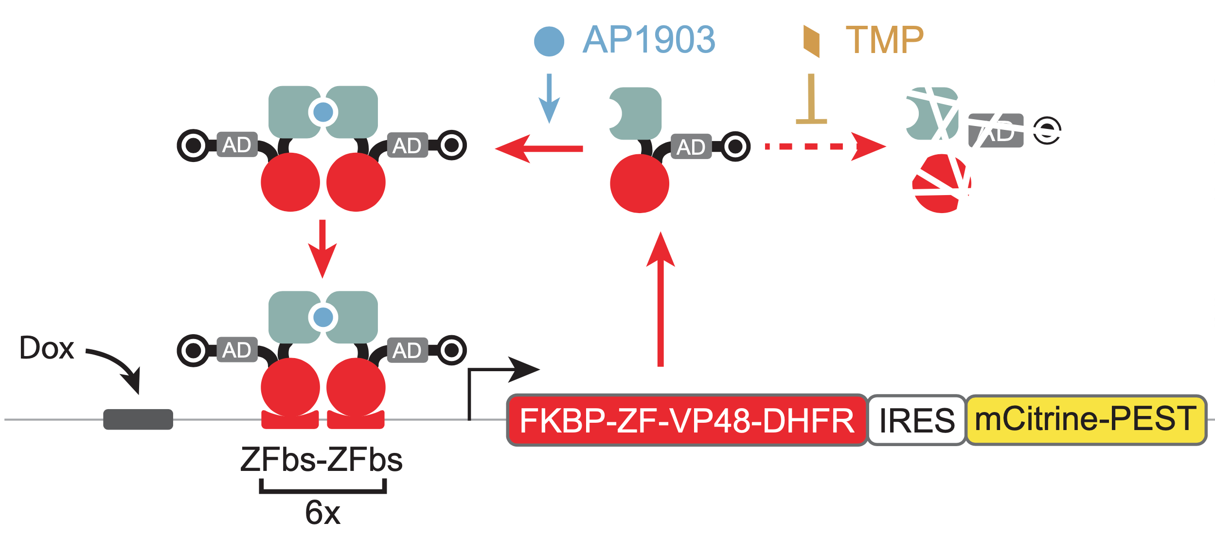
To enable systematic exploration of different parameter regimes, one would ideally like to be able to directly modulate key parameters, such as dimerization strength, protein stability, and “leaky” basal transcription, using small molecules as “control knobs.” The authors added three such knobs to the system. * First, as a dimerization domain, they used an FKBP variant that dimerizes only in the presence of the drug AP1903. This allows one to control the effective binding affinity \(K_d\) by varying the AP1903 concentration in the media. * Second, they attached a modular degron from the Dihydrofolate reductase (DHFR) protein (bullseye shape in diagram). This degradation signal targets the proteins for degradation, but can be inhibited by the small molecule antibiotic, trimethoprim (TMP). Thus, the concentration of TMP in the media controls the stability of the transcription factors. (Note that in the nondimensionalized model, \(\delta\) is lumped into the nondimensional parameters \(\tilde{\alpha} \leftarrow \alpha/(K_M \delta)\) and \(\tilde{\beta} \leftarrow \beta/(K_M \delta)\), so that modulating the protein’s degradation corresponds to scaling \(\tilde{\alpha}\) and \(\tilde{\beta}\) by the same factor.) * Third, they engineered a direct “override” into the circuit, through which one can force expression of the transcription factor. This was implemented with binding sites for standard inducible proteins just upstream of the zinc finger binding sites.
In addition to controlling these components, one also would like to read out their concentrations. For this purpose, a fluorescent protein such as mCitrine was incorporated downstream of the gene.
This diagram visually summarizes the design of one of a MultiFate transcription factor cassette.
Testing MultiFate
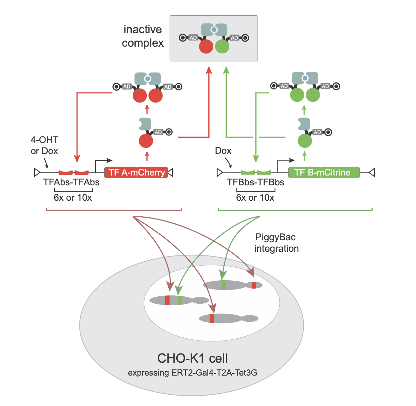
To test out the circuit, Zhu et al integrated two such cassettes with two distinct zinc finger proteins and fluorescent proteins (the greenish mCitrine and the red mCherry) into cells. Different cells received different numbers of copies of these genes integrated at different locations. In this way, each cell and its clonal descendants probed different values of the \(\alpha\) and \(\beta\) parameters for each of the two genes.
With these cells, the moment of truth was at hand: would MultiFate-2 provide multistability? When the cells were cultured without the inducers, both proteins were quite low, as seen in flow cytometry measurements. But when AP1903 and TMP were added to turn on dimerization and stabilize the proteins—voila!—the cells shifted into three distinct clusters:
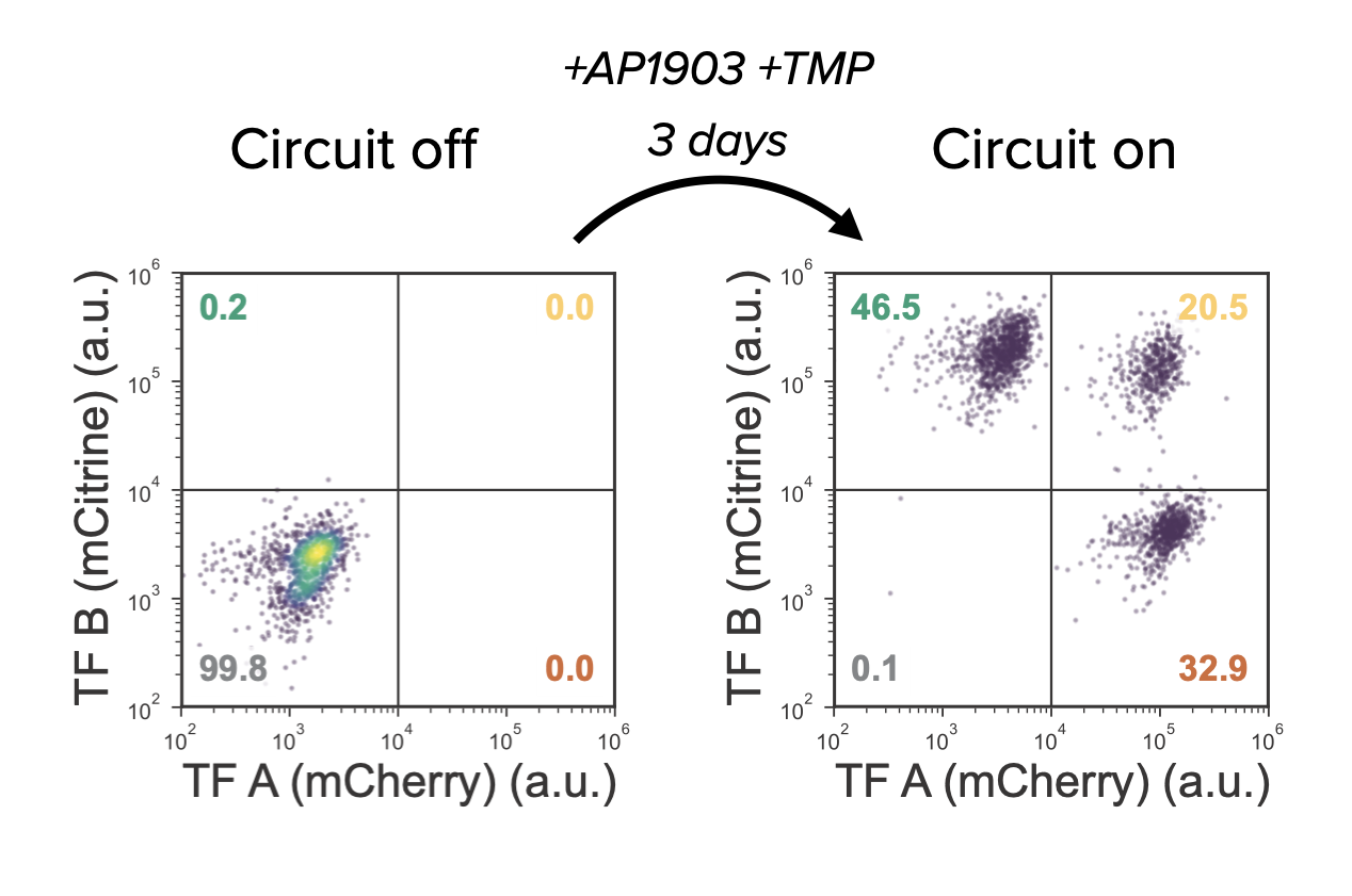
This looked eerily similar to the tristable regime described in the model!
But the appearance of three clusters alone does not prove tristability. To rigorously test stability, cells in each cluster were sorted out and cultured continuously, with periodic analysis of the distribution. If they are stable, then the distribution should not change over time. This is indeed what happened:
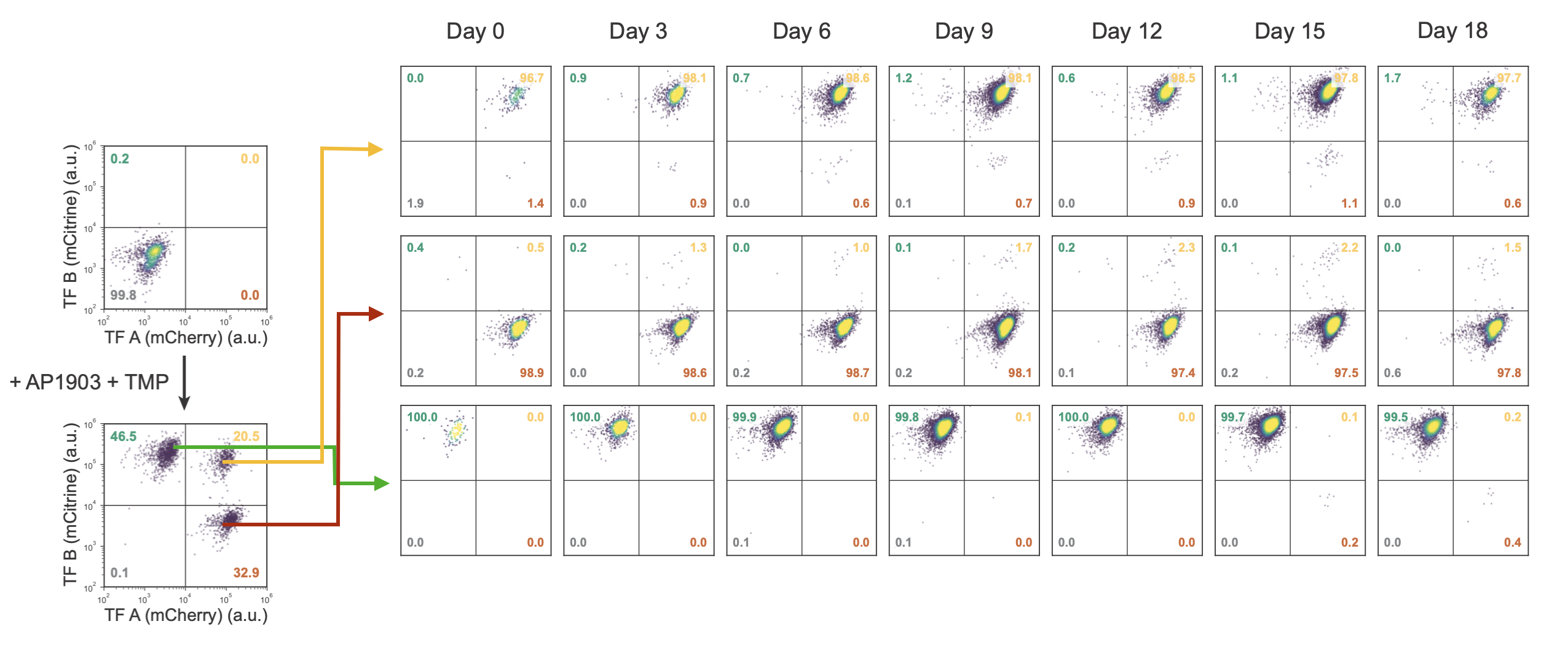
This behavior is most directly visualized in the following movie, in which individual cells in each of the three states were plated down together. Cells in the A-only and B-only states are shown in green and red, while cells in the AB state have a combination of both colors and appear yellow. You can see directly how the state (color) is faithfully preserved as cells grow into colonies.
Evidently, MultiFate-2 can indeed produce tristability. And other MultiFate-2 clones produced other behaviors as well.
Irreversible differentiation (hysteresis)
A striking feature in natural cell fate control systems is the appearance of irreversible or hysteretic transitions, in which a cell can differentiate into one or more new fates, perhaps in response to a signal, but does not (under normal conditions) de-differentiate back to its previous state. One of the best studied examples of this is the maturation of Xenopus oocytes in response to the hormone progesterone, beautifully studied by James Ferrell and colleauges. Another example is the differentiation of embryonic stem cells.
MultiFate can produce a similar type of irreversible differentiation.
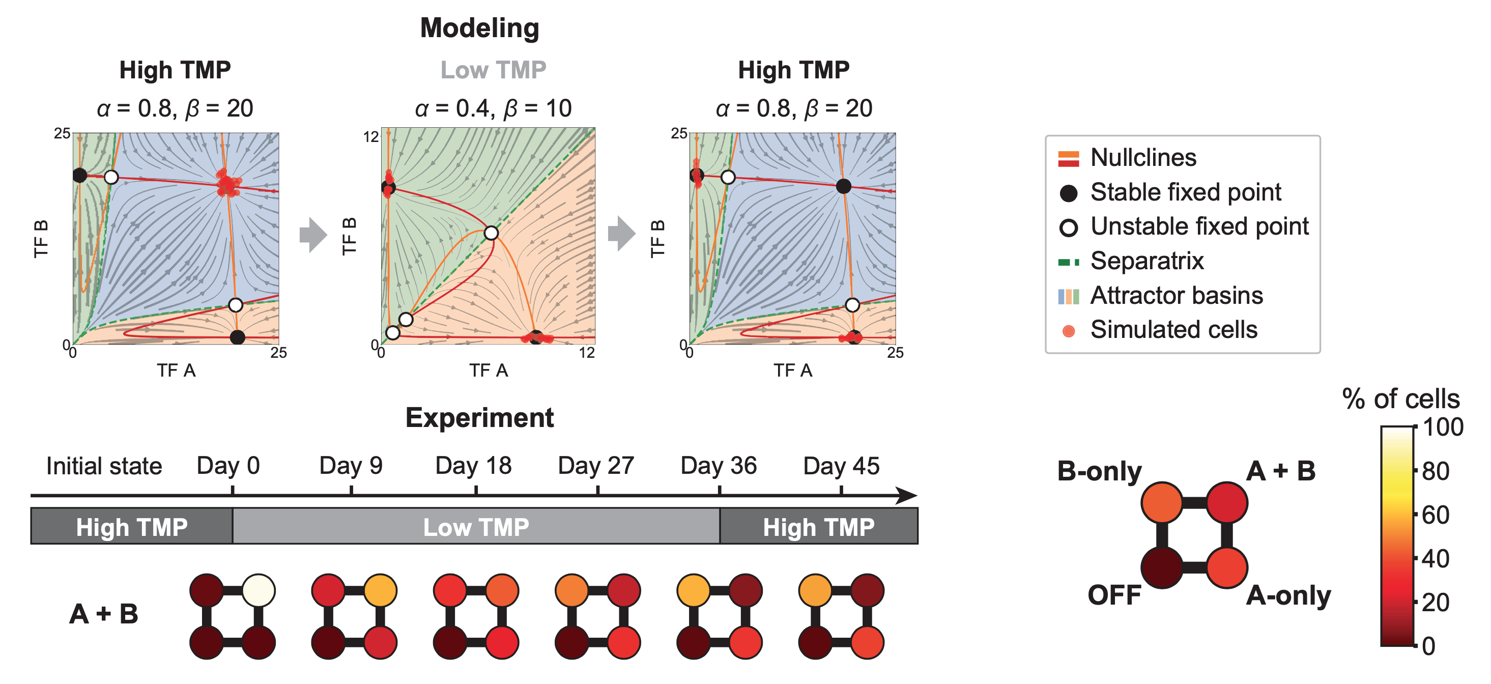
Reducing the stability of the proteins (increasing \(\delta\) in the model) produces a bistable regime, with A-only and B-only attractors but no AB attractor. Imagine starting in the AB state of the tristable regime (high TMP), and then transiently switching to the bistable regime, by reducing TMP concentration to destabilize the transcription factors. What happens? The AB cells which were happily populating a stable attractor suddenly find themselves in an unstable situation. The only attractors in the system now have A or B expression but not both. With no other choice, the cells will go to one or the other of these two states. Later, if we restore the system to the tristable regime, the AB attractor comes back. But the cells do not. They remain stuck in their new A-only and B-only states. All of this is best seen through an animation of the model:
Remarkably, the same behavior occurs in the real cells as well. In the following diagram, the four circles represent the fraction of cells in states that have low or high expression of gene A (x-axis) or B (y-axis). You can see the AB state depopulating at low TMP and not re-populating when TMP is restored.
MultiFate expands
Three states is nice. Seven states is nicer. One of the key advantages of the MultiFate architecture is that it can be expanded by plugging in additional transcription factors to an existing circuit. This works because all of the interactions between factors occur at the protein level (rather than through transcriptional regulation).
The model for MultiFate-3 can be obtained by extending the MultiFate-2 model in a straightforward way. First, we add one new differential equation for the third transcription factor, \(C\), exactly like those for \(A\) and \(B\):
\begin{align} \frac{\mathrm{d}[A_{tot}]}{\mathrm{d}t} &= \alpha + \frac{\beta [A_2]^n}{1 + [A_2]^n} - [A_{tot}] \\ \frac{\mathrm{d}[B_{tot}]}{\mathrm{d}t} &= \alpha + \frac{\beta [B_2]^n}{1 + [B_2]^n} - [B_{tot}] \\ \frac{\mathrm{d}[C_{tot}]}{\mathrm{d}t} &= \alpha + \frac{\beta [C_2]^n}{1 + [C_2]^n} - [C_{tot}] \end{align}
Second, we modify the protein dimerization expressions. This turns out to be easy because the new factor, \(C\), enters the dimerization equations exactly the same way as \(A\) and \(B\). Wherever we had \([A_{tot}] + [B_{tot}]\) above, we throw in \([C_{tot}]\) as well:
\begin{align} [A_2] &= \frac{2[A_{tot}]^2}{K_d + 4\left( [A_{tot}] + [B_{tot}] + [C_{tot}] \right) + \sqrt{K_d^2 + 8\left([A_{tot}] + [B_{tot}] + [C_{tot}]]\right)K_d}} \\ [B_2] &= \frac{2[B_{tot}]^2}{K_d + 4\left( [A_{tot}] + [B_{tot}] + [C_{tot}] \right) + \sqrt{K_d^2 + 8\left([A_{tot}] + [B_{tot}] + [C_{tot}]]\right)K_d}} \\ [C_2] &= \frac{2[C_{tot}]^2}{K_d + 4\left( [A_{tot}] + [B_{tot}] + [C_{tot}] \right) + \sqrt{K_d^2 + 8\left([A_{tot}] + [B_{tot}] + [C_{tot}]]\right)K_d}} \\ \end{align}
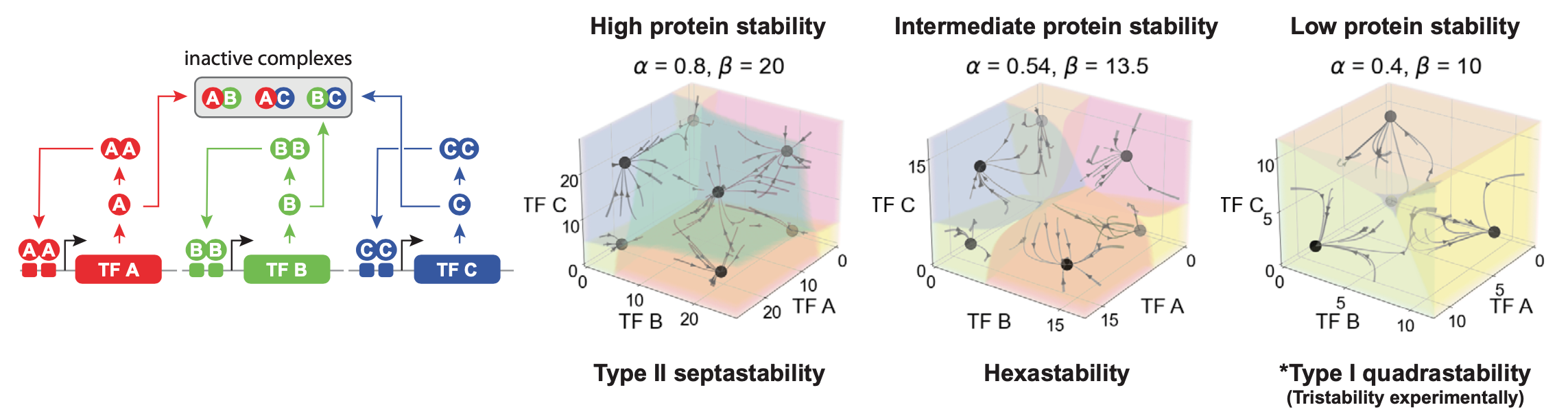
Of course, we now have a 3D phase diagram, which can be more difficult to visualize. In the following animation, the 3D diagram with shaded basins of attraction is shown in a rotating view. One can see that for the same parameters that produced tristability in MultiFate-2, we now have septastability (7 states) with MultiFate-3. The states include single transcription factor expression, all pairs, and a state with all three factors on simultaneously:
Does this really happen? To find out, Zhu et al added a third zinc finger, in a third color (displayed in the blue channel) to the existing MultiFate-2 circuit. Indeed, all 7 predicted states occurred, and were stable, as you can see in this movie, where the three proteins are displayed in the red, green, and blue channels and each state therefore has a unique color combination:
MultiFate-3-MovieS5_MF3movie.mp4
Having demonstrated that a 2-gene MultiFate circuit exhibits the desired stability and controllability properties for a differentiation circuit, Zhu et al. then demonstrated the MultiFate architecture’s expandability by constructing and measuring the performance of a 3-gene MultiFate circuit. Through mathematical modeling they were able to determine that the 3-gene circuit could exhibit septastability (the coexistence of seven stable fixed points), and through experimental measurements they were able to determine that cells that started in each of these seven states persisted within these states for at least 18 days in the absence of external control signals.
With MultiFate, in experiments as well as in the model, the number of states increases faster than the number of transcription factors. This is essential to achieve very large numbers of states.
Progressive differentiation
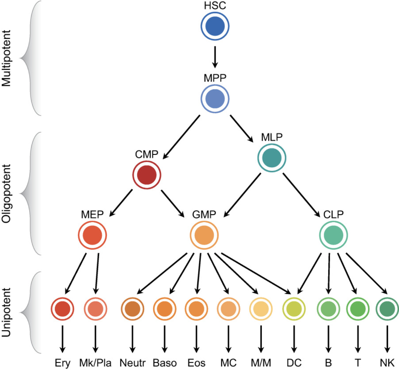
A classic theme in natural cell fate control systems is the occurrence of branching fate decisions, exemplified by this illustration of cell fate diversification in the hematopoietic system (Antoniani et al):
MultiFate-3 can perform something roughly similar. If we progressively reduce protein stability by increasing \(\delta\) in the model, then we progressively destabilize certain states, forcing binary decisions. To see this, we can plot the MultiFate-3 phase diagram at different stabilities. The following simulation starts in the full septastable regime. Then stability is suddenly reduced, eliminating the triple positive ABC state. Cells starting in that state migrate to the double positive states: AB, BC, and AC. Then, just as they are getting comfortable, we can further reduce protein stability. Now the double positive states become unstable as well, and cells migrate to the A-only, B-only, and C-only states. In this way, varyiung one parameter can cause a progressive series of decisions.
Remarkably, this occurs not only in the model but in the real system as well (see Zhu et al).
Scaling: how far can it go?
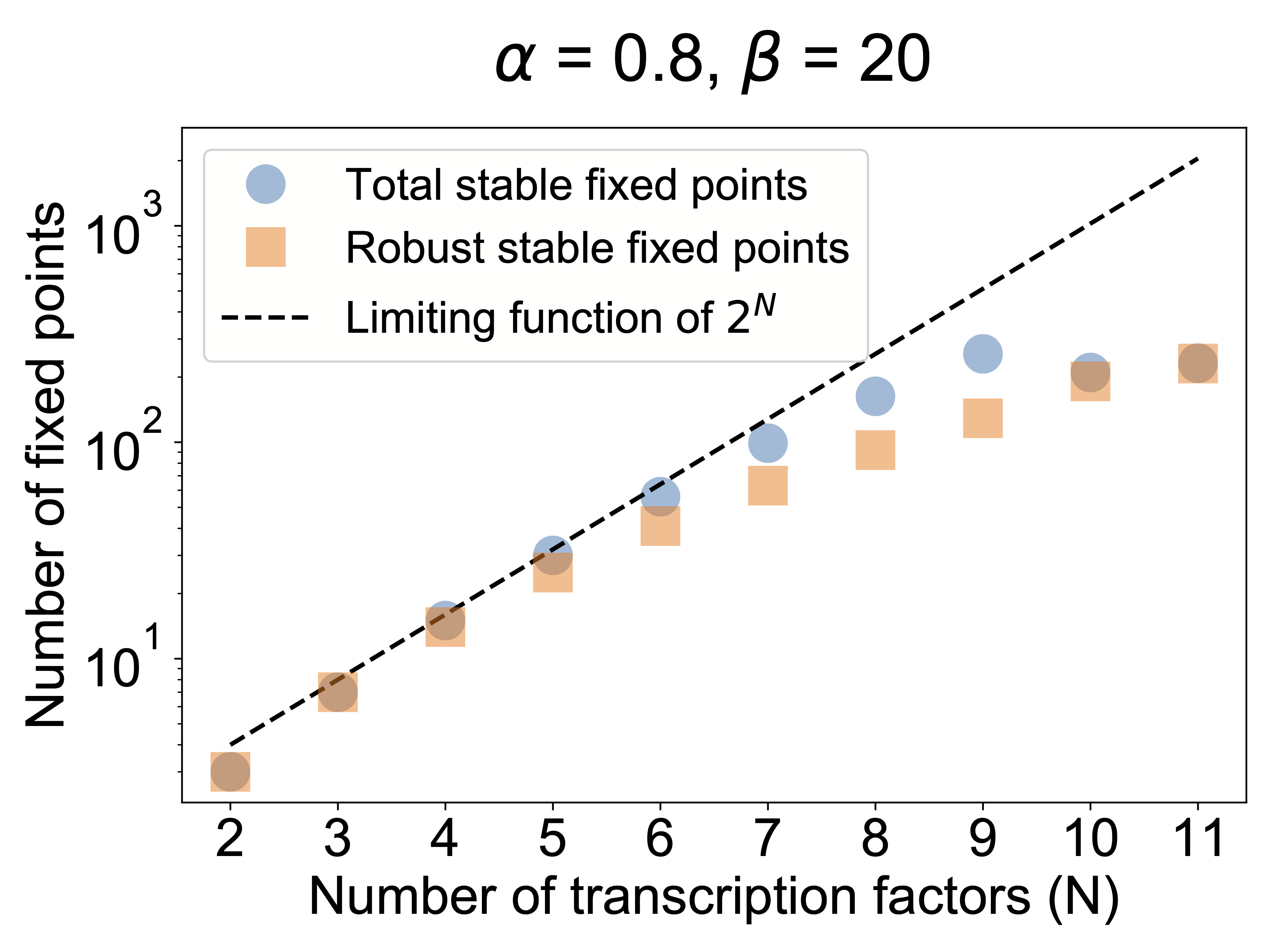
A final question we can ask in the model is how far can MultiFate scale? How many states can it generate? To address this question, one can analyze MultiFate models with increasing numbers of transcription factors. In addition to counting the number of stable fixed points, we can also quantify the relative sizes of their basins of attraction to make sure they are really accessible. Zhu et al performed this analysis. As shown in the next plot, the number of states initially grows exponentially with the number of factors. Eventually it starts to saturate. The reason for this turns out to be interesting. In the MultiFate architecture, only the homodimers are active. For a state with a certain number, \(m\) of transcription factors simultaneously expressed, there are \(~m^2\) dimer complexes but only \(m\) of those are active. So the fraction of all species that are active decreases as \(~1/m\). This eventually limits the total number of states. Nevertheless, for the parameters in the model, it still reaches hundreds of states!
It will be interesting to see how far MultiFate can scale, which aspects of MultiFate occur in natural fate control systems, and what advantages other architecture might also provide.
Conclusion
Multicellular organisms are built from multiple cells in multiple states. Understanding how those states are established, stabilized, and controlled remains a fundamental biological challenge. Natural circuits appear to combine combinatorial dimerization and positive autoregulation—two circuit level features we have already encountered. The synthetic MultiFate circuit shows that these two features together provide a scalable architecture for multistability with many features that are reminescent of natural cell fate control systems. Additional mechanisms are almost certain to play critical roles. Nevertheless, this approach reveals that multistability can be engineered, and provokes a range of questions about how combinations of transcription factors work to specify fates and their transitions. Above, the knobs used to experimentally control the state of the MultiFate circuit were external, based on small molecules. In future iterations, a larger circuit may be able to control these dynamics autonomously or in response to signals from other cells, similar to the behaviors observed during the development of multicellular organisms. Achieving this vision will likely require uncovering additional design principles for multicellularity.