Problem 13.1: Programming cellular response
[1]:
import numpy as np

import eqtk
We have seen in this chapter that the combinatoric binding of multiple ligand types with multiple receptor types can lead to cellular addressing. In this problem, you will develop a scheme using two types of ligands, two types of “A” receptors, and two types of “B” receptors whereby the cell can respond to variation in ligand concentration in three orthogonal prescribed ways. These responses vary based on concentration of the respective receptors; the expression of these receptors delineate cell types.
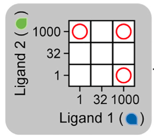
In our approach, we will closely follow the work of Su, et al., 2022. We use the one-step promiscuous ligand-receptor model from this chapter, using the same notation. We define by a ligand “word” to be a set of specific concentration values for each ligand variant in a combination. For example, a concentration of 10 mM for ligand 1 and 100 mM for ligand 2 constitutes a ligand word (10 mM, 100 mM). In the diagram below, we have three ligand words denoted by the red circles, (1, 1000), (1000, 1), and (1000, 1000).
Each word should encode a separate cellular response, giving different cell types. An example of three responses is shown in the image below.
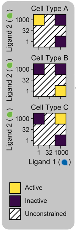
The cell “cares” about the levels in the colored regions; the response in the hatched regions is irrelevant. In the above diagram, purple indicates low response and yellow indicates a high response.
Your task is to come up with a set of parameters, eight \(K_{ijk}\)’s and eight \(\epsilon_{ijk}\)’s, along with three sets of receptor concentrations, each containing the concentrations of A₁, A₂, B₁, and B₂, that have the desired response above, one each for each of the three words (1, 1000), (1000, 1), and (1000, 1000). An example of a desired response is shown below.
In working this problem, it helps to have some handy functions from the chapter.
[2]:
def make_rxns(nA, nB, nL):
    '''
    Generate trimolecular binding reactions for a system with
    nA, nB, and nL types of Type A receptors, Type B receptors,
    and ligands, respectively. Returns a single string.
    '''
    rxns = ""
    for k in range(nB):
        for j in range(nL):
            for i in range(nA):
                rxns += f"A_{i+1} + L_{j+1} + B_{k+1} <=> T_{i+1}_{j+1}_{k+1}\n"
    return rxns


def make_N(nA, nB, nL):
    """Generate a stoichiometric matrix for ligand-receptor binding with
    nA, nB, and nL types of Type A receptors, Type B receptors, and
    ligands, respectively.
    """
    rxns = make_rxns(nA, nB, nL)
    N = eqtk.parse_rxns(rxns)

    # Sorted names
    names = sorted(N.columns, key=lambda s: (len(s), s))

    # Sorted columns
    N = N[names]

    # As a Numpy array
    return N.to_numpy(copy=True, dtype=float)


def readout(epsilon, c):
    """Readout function of a set of complex concentrations. This
    is the expression level of the genes under regulation of
    singaling from the receptors.
    """
    return np.dot(epsilon, c[:, -len(epsilon):].transpose())
[25]:
print(make_rxns(2, 2, 2))
A_1 + L_1 + B_1 <=> T_1_1_1
A_2 + L_1 + B_1 <=> T_2_1_1
A_1 + L_2 + B_1 <=> T_1_2_1
A_2 + L_2 + B_1 <=> T_2_2_1
A_1 + L_1 + B_2 <=> T_1_1_2
A_2 + L_1 + B_2 <=> T_2_1_2
A_1 + L_2 + B_2 <=> T_1_2_2
A_2 + L_2 + B_2 <=> T_2_2_2
We can make a stoichiometric matrix using these functions; it will be the same for all calculations we do.
[36]:
N = make_N(2, 2, 2)
Half of the battle in problems like these is keeping track of indices to know what species is what. The columns of the stoichiometric matrix correspond to the following species.
index |
species |
|---|---|
0 |
A₁ |
1 |
A₂ |
2 |
B₁ |
3 |
B₂ |
4 |
L₁ |
5 |
L₂ |
6 |
A₁L₁B₁ |
7 |
A₂L₁B₁ |
8 |
A₁L₂B₁ |
9 |
A₂L₂B₁ |
10 |
A₁L₁B₂ |
11 |
A₂L₁B₂ |
12 |
A₁L₂B₂ |
13 |
A₂L₂B₂ |
These indices also correspond to the species in our inputted initial concentrations and in the output of EQTK’s solver for the equilibrium concentrations. With that in mind, we can write a function to generate our initial concentration values for a given set of initial ligand concentrations, cL0.
[30]:
def make_c0_grid(cL0, cA10, cA20, cB10, cB20):
    """Create an array of initial concentrations.

    Parameters
    ----------
    cL0 : array_like
        Array of ligand concentrations. This is the same for ligand
        1 and ligand 2, so a single 1D array is all that is required.
    cA10 : float
        Total concentration of receptor A1.
    cA20 : float
        Total concentration of receptor A2.
    cB10 : float
        Total concentration of receptor A1.
    cB20 : float
        Total concentration of receptor B2.

    Returns
    -------
    output : 2D Numpy array
        If n is the length of the cL0 input array, the output
        is an n² by 14 array. Columns 0 through 3 are the total
        receptor concentrations. Columns 4 and 5 are the ligand
        concentrations. Columns 6 through 13 are the concentrations
        of all of the possible trimers (all set to zero).
    """
    # Number of ligand concentrations
    n = len(cL0)

    # Ligand concentrations
    cL0 = np.meshgrid(*tuple([cL0] * 2))

    # Initialize c0
    c0 = np.zeros((n**2, 14))

    # Add ligand concentrations
    c0[:, 4] = cL0[0].flatten()
    c0[:, 5] = cL0[1].flatten()

    # Add receptor concentrations
    c0[:, 0] = cA10
    c0[:, 1] = cA20
    c0[:, 2] = cB10
    c0[:, 3] = cB20

    return c0
In trying to find parameters, we will use the ligand concentrations below.
[31]:
cL0 = np.array([1.0, 32.0, 1000.0])
Next, in order to do the calculation, we need to specify the prescribed target response of the various cell types and for which ligand words the target response is relevant (ignoring the hatches areas in the graphic above). We refer to the latter as active_words, defined below.
[33]:
# Ligand words from top diagram
active_words = np.array([0, 0, 1, 0, 0, 0, 1, 0, 1], dtype=bool)
You can see how it corresponds to the words by comparing to our target ligand concantrations.
[34]:
c0 = make_c0_grid(np.array([1, 32, 1000]), 0, 0, 0, 0)
print("Ligand 1:    ", c0[:, 4])
print("Ligand 2:    ", c0[:, 5])
print("active words:", active_words)
Ligand 1:     [   1.   32. 1000.    1.   32. 1000.    1.   32. 1000.]
Ligand 2:     [   1.    1.    1.   32.   32.   32. 1000. 1000. 1000.]
active words: [False False  True False False False  True False  True]
We can now specify a list of target responses.
[35]:
targets = [
    np.array([0, 0, 0, 0, 0, 0, 1, 0, 0]), # Ligand 1 low, ligand 2 high
    np.array([0, 0, 1, 0, 0, 0, 0, 0, 0]), # Ligand 1 high, ligand 2 low
    np.array([0, 0, 0, 0, 0, 0, 0, 0, 1]), # Ligand 1 high, ligand 2 high
]

# Useful to know how many cell types we have
n_cell_types = len(targets)
Finally, it will be useful to have a function to solve for the normalized response of a cell to an inputted set of initial concentrations and parameters. The function returns the cellular response, with the maximum value of the response over all ligand concentrations being set to one. That is, we want a function that returns \(s_\mathrm{norm}\), defined by
\begin{align} &s(l_1, l_2) = \sum_{ijk} \epsilon_{ijk}\,t_{ijk}(l_1, l_2),\\[1em] &s_\mathrm{norm}(l_1,l_2) = \frac{s(l_1, l_2)}{\text{maximal }s\text{ over all ligand concentrations}}. \end{align}
a) Complete the function below.
[9]:
def solve_norm_response(c0, N, K, epsilon):
    """Solve for normalized response. Returns a one-dimensional array
    containing signal levels corresponding to each row in `c0`.
    """
    pass
b) To find optimal parameters that give cell responses close to the target responses, you can use whatever method you like. However, we will walk you through a method following Su, et al., which you may find easier to do that developing your own method.
We will use a least squares method. To do this we define a residual, which is the value of the signal a given active ligand word, minus the target signal for that word.
\begin{align} \text{residual}(l_1, l_2) = s_\mathrm{norm}(l_1, l_2) - s_\mathrm{norm}^\mathrm{target}(l_1, l_2). \end{align}
We then seek to minimize the sum of these residuals. Note that there exists three residuals for each cell type in the above example, for a total of nine residuals.
The scipy.optimize.least_squares() function performs this calculation automatically. Its call signature is
scipy.optimize.least_squares(residuals, x0, bounds=(lower_bounds, upper_bounds), args=args)
Here, residuals() is a function that returns the array of residuals and has call signature
residuals(x, *args),
where x is an array of the parameters being optimized and args is a tuple of any other arguments the function needs. To keep things organized, we will take the first eight entries in x to be the \(K_{ijk}\) values, the next eight entries to be the \(\varepsilon_{ijk}\) values, and the remaining twelve entries to be the receptor concentrations for the respective cell types.
Complete the function below.
[10]:
def residuals(x, cL0, targets, active_words, N):
    """Return array of residuals."""
    # Unpack x, log K's, then log epsilons, then receptor concs
    K = x[:8]
    epsilon = x[8:16]
    receptor_conc = x[16:]

    pass
Given our function residuals, we can define args to match its call signature.
[11]:
args = (cL0, targets, active_words, N)
c) To complete the optimization, we need to two more pieces. First, we need to provide bounds for all of the parameters. All of the \(K_{ijk}\), \(\varepsilon_{ijk}\), and receptor concentrations must be positive, so we have the following for the lower bounds.
[12]:
lower_bounds = np.zeros(16 + 4 * n_cell_types)
For the upper bounds, Su, et al., specified that all \(K_{ijk}\) and \(\varepsilon_{ijk}\) must be between zero and one. This effectively sets the arbitrary units of the ligand and receptor concentrations. (We do not require that the sum of the \(K_{ijk}\)’s and the sum of the \(\varepsilon_{ijk}\)’s sum to one.) The receptor concentrations are unbounded, so we can set the upper bounds, recalling the ordering of our parameter array.
[13]:
upper_bounds = np.concatenate(
    (
        np.ones(16),  # Upper bounds on K's and ε's
        np.inf * np.ones(4 * n_cell_types) # Upper bounds on receptor concs
    )
)
Finally, we must provide a guess of the parameter values. Su, et al. used the strategy that the initial guess of all receptor concentrations were one and randomly chose values for \(K_{ijk}\) and \(\epsilon_{ijk}\) from a uniform distribution on the interval [0, 1]. You can try this strategy as in the code cell below or adopt one of your own.
[14]:
# Initial guesses of parameter values
K0 = np.random.uniform(size=8)
epsilon0 = np.random.uniform(size=8)
receptor_conc0 = np.ones(4 * n_cell_types)

# Package together
x0 = np.concatenate((K0, epsilon0, receptor_conc0))
Now, you can perform the optimization be running
res = scipy.optimize.least_squares(
    residuals, x0, bounds=(lower_bounds, upper_bounds), args=args
)
The object return is the optimization result. You can pull out the parameter values from the res.x attribute.
K = res.x[:8]
epsilon = res.x[8:16]
receptor_conc = res.x[16:]
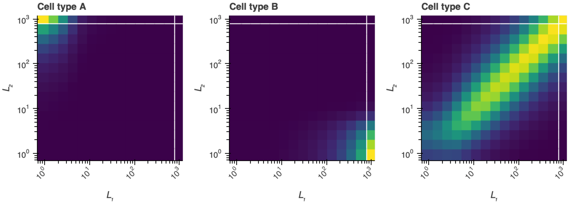
Find a set of parameters that give the desired cell types. Make a plot like the triptych above for the various cell types to demonstrate that you parameter set does indeed give the desired orthogonal cell types. Also report the respective receptor concentration profiles of each of the three cell types.
Hint: The optimization will converge to a local minimum, which may not hit your target addressing very well. There are lots of local minima. You can try rerunning the optimization with a different set of starting guesses for the parameters and receptor concentrations. You may have to do this several times.
d) If you like, try coming up with parameter values for other word sets and/or target responses.
[46]:
c0

# Set up fixed concentrations
fixed_c = -np.ones_like(c0)
fixed_c[:, 4:6] = c0[:, 4:6]

# # Solve for the concentrations
# c = eqtk.fixed_value_solve(c0=c0, fixed_c=fixed_c, N=N, K=K)

# # Build and return normalized response
# s = readout(epsilon, c)
[49]:
c0.shape
[49]:
(9, 14)
[47]:
fixed_c
[47]:
array([[  -1.,   -1.,   -1.,   -1.,    1.,    1.,   -1.,   -1.,   -1.,
          -1.,   -1.,   -1.,   -1.,   -1.],
       [  -1.,   -1.,   -1.,   -1.,   32.,    1.,   -1.,   -1.,   -1.,
          -1.,   -1.,   -1.,   -1.,   -1.],
       [  -1.,   -1.,   -1.,   -1., 1000.,    1.,   -1.,   -1.,   -1.,
          -1.,   -1.,   -1.,   -1.,   -1.],
       [  -1.,   -1.,   -1.,   -1.,    1.,   32.,   -1.,   -1.,   -1.,
          -1.,   -1.,   -1.,   -1.,   -1.],
       [  -1.,   -1.,   -1.,   -1.,   32.,   32.,   -1.,   -1.,   -1.,
          -1.,   -1.,   -1.,   -1.,   -1.],
       [  -1.,   -1.,   -1.,   -1., 1000.,   32.,   -1.,   -1.,   -1.,
          -1.,   -1.,   -1.,   -1.,   -1.],
       [  -1.,   -1.,   -1.,   -1.,    1., 1000.,   -1.,   -1.,   -1.,
          -1.,   -1.,   -1.,   -1.,   -1.],
       [  -1.,   -1.,   -1.,   -1.,   32., 1000.,   -1.,   -1.,   -1.,
          -1.,   -1.,   -1.,   -1.,   -1.],
       [  -1.,   -1.,   -1.,   -1., 1000., 1000.,   -1.,   -1.,   -1.,
          -1.,   -1.,   -1.,   -1.,   -1.]])