1. Introduction to biological circuit design
Concepts
Biological circuits are sets of interacting molecular or cellular components that implement and control cellular behaviors.
Circuit design principles relate a feature of a circuit to the function it provides for the cell. They often take the form Feature X enables Function Y.
Design principles can help explain why and when one circuit design or architecture would be preferred over another.
A simple design question is when to use positive activation or negative repression to regulate a gene.
Techniques
Ordinary differential equations for protein production and removal allow analysis of simple gene expression processes.
Separation of time-scales simplifies circuit analysis.
Gene regulation circuits can be analyzed in terms of binding of activators and repressors to binding sites in the promoter region.
Executable Jupyter notebooks (like this one) enable interactive exploration of key concepts.
[1]:
# Colab setup ------------------
import os, sys, subprocess
if "google.colab" in sys.modules:
    cmd = "pip install --upgrade watermark"
    process = subprocess.Popen(cmd.split(), stdout=subprocess.PIPE, stderr=subprocess.PIPE)
    stdout, stderr = process.communicate()
# ------------------------------

import numpy as np
import bokeh.io
import bokeh.plotting

bokeh.io.output_notebook()
Biological circuit design
The living cell is a device unlike any other: It can sense its environment, search out nutrients, avoid threats, control its own division and growth, while quietly keeping track of time. Individual cells can switch into a multitude of different states, coordinate with other cells to build complex multicellular tissues and organs (even brains!), develop into social organisms, and generate immune systems that can patrol those organisms to repair damage and destroy pathogens. Most of the time, they do these things reliably, with minimal external help, and without complaining. How are these incredible behaviors programmed within the cell? Can we understand cells well enough to rationally predict, control, or even reprogram their behaviors?
In this book, we will develop foundational concepts, approaches, and examples that will enable us to address these critical biological challenges. The key premise is that many of these problems can be addressed by thinking of biological systems in terms of circuits – sets of molecular or cellular components that interact with another in specific ways.
What is a biological circuit?
We will consider two levels of biological circuitry:
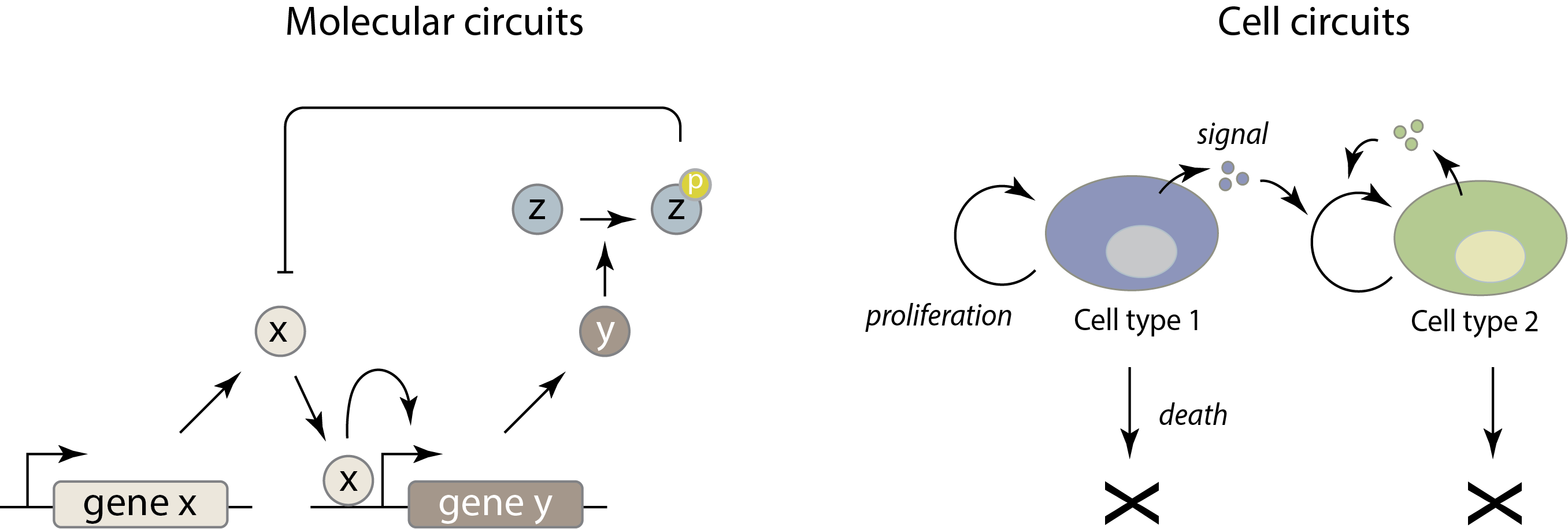
Molecular circuits consist of molecular species (genes, proteins, etc.) that interact with, and regulate, one another in specific ways. For example, a given gene can be transcribed to produce a corresponding mRNA, which can in turn be translated to produce a specific protein. That protein may be a repressor that turns off expression of a different gene, or even its own gene. Similarly, a protein kinase may phosphorylate a specific target protein, altering its ability to catalyze a reaction or modify another protein. The molecular specificity of these interactions—analogous to wires in electronics—is the key property that enables them to form molecular circuits. Molecular circuits represent a fascinating level of cellular organization, midway between the inanimate chemistry of molecules, and the fully “alive” state of a complete cell.
One level up, we will also consider cell circuits. In this case, cells in different states, of different types, or even from different species signal to one another to control each other’s growth, death, proliferation, and differentiation. The key variables in these circuits are the population sizes and spatial arrangements of each type of cell. For example, in the immune system, different cell types influence each other’s proliferation and differentiation through cytokines and other signals, forming a collection of complex, interconnected cell circuits.
The two levels are not independent. The behavior of each cell type within a cell circuit is determined by the structure of its molecular circuits.
At both levels, as we explore different circuits, we will approach them from a design point of view, seeking to understand the tradeoffs among alternative circuit designs, and looking for design principles that explain why and in what context one design might be preferred over another. These design principles can help to make sense of an otherwise bewildering space of potential circuits.
There are several wonderful aspects to working at the circuit level: First, circuits are particularly amenable to experimental analysis. If we want to know how one element of a circuit, whether a protein or a cell type, affects another, we can directly perturb it and observe the responses of other components. In other words, we can play with circuits. Second, circuits can be engineered. We can design and construct many different synthetic circuits from a handful of components and compare their behavior. This provides a way to experimentally explore the behavior of different circuit designs, even those that do not occur naturally, directly within living cells. Third, circuits can be modeled. Once we know how a set of components behave, we can generate testable predictions for how circuits comprised of those components ought to behave. Thus, circuits are an arena in which analysis, synthesis, and modeling come together in a beautiful way.
From molecular biology to systems biology
Historically, the framework of molecular biology became dominant in the second half of the twentieth century, with the central idea that we could understand biological phenomena in terms of the molecular structure and biochemical function of DNA, mRNA, and other molecules. (The Eighth Day of Creation by Horace Freeland Judson provides a riveting history of molecular biology.) Despite the focus on individual molecules, it was clear to the pioneers of molecular biology that all of these molecules functioned together in circuits. For example, in a 1962 essay, speaking about the organization of transcriptional regulatory systems, Jacob and Monod wrote,
It is obvious from the analysis of these [bacterial genetic regulatory] mechanisms that their known elements could be connected into a wide variety of ‘circuits’ endowed with any desired degree of stability.
During the 2000s, interest in the structure and function of circuits began to explode, fueled in part by new technologies that enabled quantitative, high-throughput, top-down “omic” measurements of biological systems. Researchers could suddenly analyze the expression of not just a few genes in the cell, but nearly all of them at once, and see how they vary over time or in response to different conditions. But data don’t analyze themselves, and it was not always clear how to to use these large scale data sets to predict, let alone understand, cellular behaviors. At the same time, more traditional, bottom-up analyses of specific cellular processes had accumulated detailed information on many individual genes and proteins and their interactions. As more components and interactions were identified, the limitations of reasoning directly from cartoons of positive and negative arrows became clear, highlighting the challenge of understanding how components function together cohesively as a circuit. Somehow, a new field seems to have emerged, loosely defined by its focus on the circuit level, but diverse in its approaches and subject matter. It took the name systems biology.
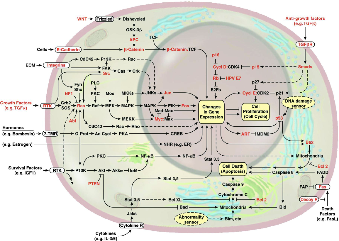
*This image of the cell as a set of circuits comes from a classic review of cancer Hanahan and Weinberg, 2000.
Designing biological circuits
Circuit design problems emerge whenever one can build many different products from arrangements of the same elements. Electronic circuits are composed of a handful of different kinds of elements: transistors, resistors, capacitors, etc. that can be connected in different ways to produce circuits with different properties. Design requires comparing different circuit designs that may appear to perform similar functions, but in fact exhibit different tradeoffs, e.g. between power and performance, or speed and precision. Design problems are also prevalent outside of science and engineering. For example, to make a movie poster one has to choose and arrange graphical elements in relation to one another.
We now have much information about the molecular components of cells (genes, RNAs, proteins, metabolites, and many other molecules) and their interactions. In many cases, we know the sites at which transcription factors bind genome-wide, which proteins chemically modify which others, and which proteins function together in complexes. It might seem as if we ought to already be able to understand, predict, and control cellular circuits with great precision. However, fundamental questions about the designs of these circuits still remain unclear. For example:
What capabilities does each circuit provide for the cell? (function, design principles)
What features of circuit architecture enable these ? (mechanism)
How can we control cells in predictable ways using these circuits? (biomedical applications)
How can we use circuit design principles to program predictable new behaviors in living cells? (synthetic biology and bioengineering)
Similar principles apply to natural and synthetic circuits.
In this book, we will address these questions for both natural and synthetic circuits. The former are discovered in microbes, plants, and animals, while the latter are designed and engineered in cells out of well-characterized, re-engineered, or de novo designed genes, proteins, and other molecular components. Despite their different origins, natural and synthetic circuits, operating in similar biological contexts, should share a common set of design principles. That is, the principles that allow a circuit to function effectively within or among cells do not necessarily depend on whether that circuit evolved naturally or was designed and constructed in the lab. Having said that, we also recognize that evolution may be able to produce designs that are more complex or different from those we are currently able to construct, or even conceive, and that we do not in most cases understand all of the constraints impacting natural circuits. A major theme of this book is that principles from natural circuits can often allow more effective synthetic circuit design.
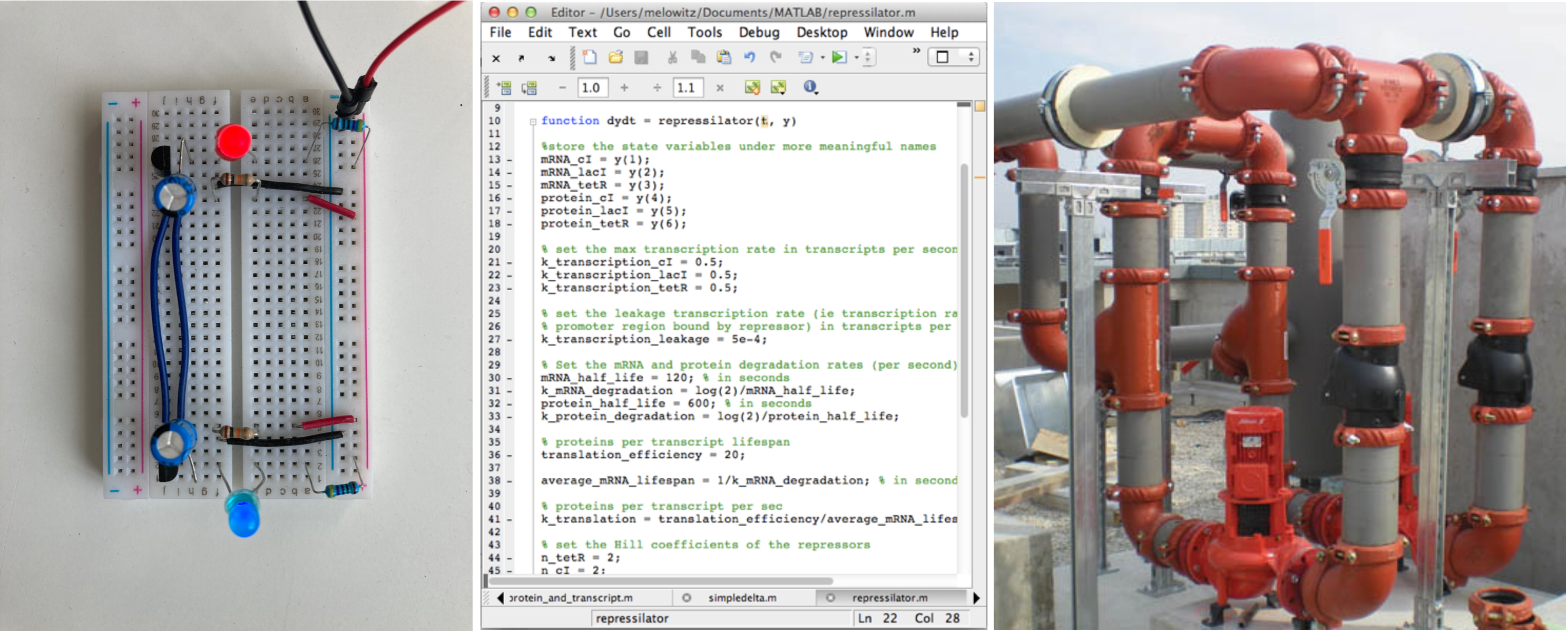
Electronics, software, and plumbing are great examples of human-designed systems that possess many properties analogous to biological circuits. These systems are based on known design principles that sometimes overlap with, and sometimes differ from, those of biological circuits. Plumbing picture by flickr user frozen-tundra,CC-BY-2.0 licensed.
Biological circuits differ from many other types of circuits or circuit-like systems
Is biological circuit design a solved problem? Electronics, software, plumbing, construction, and other human designed systems are based on connections between modular components (see Figure). Can we not just apply known principles of those systems biological circuits? The answer is generally “no,” or “only a little,” because biological systems differ in fundamental ways from these systems:
Natural circuits were not designed by people. They evolved. That means they are not “well-documented” and their function(s) are often unclear.
Even synthetic circuits, which are designed by people, often use evolved components (such as proteins or protein domains) from natural proteins, which we do not fully understand.
Biological circuits use different designs than many human-engineered circuits. For example, in cells, molecular components often appear to exhibit extensive networks of promiscuous interactions (“crosstalk”) among their components, which are typically avoided in electronics, where connections are more limited. As we will see, these promiscuous interactions can provide critical capabilities.
Noise: While electronic circuits can function deterministically, biological circuits function with high levels of stochastic (random) fluctuations, or “noise,” in their own components. Noise is not just a nuisance: some biological circuits take advantage of it to enable behaviors that would not be possible without it!
Electrical systems use positive or negative voltages and currents, allowing for positive or negative effects. By contrast, biological circuits are built out of molecules (or cells) whose concentrations cannot be negative. That means they must use other mechanisms for “inverting” activities.
From a more practical point of view, we have a very limited ability to construct, test, and compare designs. Even with recent developments such as CRISPR, our ability to rapidly and precisely produce cells with well-defined genomes remains limited compared to what is possible in more advanced disciplines. (This situation is rapidly improving!)
What other fundamental differences between biological circuits and human designed systems can you think of?
Inspiration from electronics
In their classic book, The Art of Electronics, Horowitz and Hill explain something similar to the excitement many feel now about biological circuit design.
The field of electronics is one of the great success stories of the 20th century. From the crude spark-gap transmitters and “cat’s-whisker” detectors at its beginning, the first half-century brought an era of vacuum-tube electronics that developed considerable sophistication and found ready application in areas such as communications, navigation, instrumentation, control, and computation. The latter half-century brought “solid-state” electronics — first as discrete transistors, then as magnificent arrays of them within “integrated circuits” (ICs) — in a flood of stunning advances that shows no sign of abating. Compact and inexpensive consumer products now routinely contain many millions of transistors in VLSI (very large-scale integration) chips, combined with elegant optoelectronics (displays, lasers, and so on); they can process sounds, images, and data, and (for example) permit wireless networking and shirt-pocket access to the pooled capabilities of the Internet. Perhaps as noteworthy is the pleasant trend toward increased performance per dollar. The cost of an electronic microcircuit routinely decreases to a fraction of its initial cost as the manufacturing process is perfected….
On reading of these exciting new developments in electronics, you may get the impression that you should be able to construct powerful, elegant, yet inexpensive, little gadgets to do almost any conceivable task — all you need to know is how all these miracle devices work.
Indeed, the marvelous progression of electronic circuit capabilities they describe could well describe biological circuits decades from now. Like electronics, we may will soon be able to program cellular “miracle devices” to create “little gadgets” that address serious environmental and medical applications.
Premise and goals
This book explores foundational concepts needed to understand, predict, and control living systems with greater precision (systems biology), and to design synthetic circuits that provide new functions (synthetic biology). We will develop quantitative approaches for analyzing different circuit designs (tools), and also identify circuit design principles that provide insight and intuition into how different designs operate, and why they were selected by evolution or synthetic biologists.
Design principles relate circuit features to circuit functions
We will define a circuit design principle as a statement of the form: Circuit feature X enables function Y. Many chapters of the book will explore a design principle. Here are just a few examples:
Negative autoregulation of a transcription factor accelerates its response to a change in input.
A tightly binding inhibitor can threshold the activity of a target protein, enabling ultrasensitive responses.
Positive autoregulation and ultrasensitivity can enable bistability, the ability of a cell to stably exist in two distinct states.
Pulsing a transcription factor on and off at different frequencies (time-based regulation) can enable coordinated regulation of many target genes.
Noise-excitable circuits enable cells to control the probability of transiently differentiating into an alternate state.
Mutual inactivation of receptors and ligands in the same cell enable equivalent cells to signal unidirectionally.
Promiscuous (many-to-many) interactions among ligands and receptors enable cells to selectively respond to specific ligand combinations.
Independent tuning of gene expression burst size and frequency enables cells to control cell-cell heterogeneity in gene expression.
Feedback on morphogen mobility allows tissue patterns to scale with the size of a tissue.
New principles are still emerging in ongoing research.
With the general premise of the course out of the way, we can immediately start to analyze some systems:
Developing intuition: Steady state expression levels depend on protein production and removal rates.
We will start with the simplest possible “circuit”—hardly a circuit at all, really, just a single gene coding for a single protein expressed at a constant level. This minimal example will allow us to develop intuition for the dynamics of the simplest gene regulation systems and lay out a procedure that we can further extend to analyze more complex circuits.
How much protein will the gene x produce? We assume that the gene will be transcribed to mRNA and those mRNA molecules will in turn be translated to produce proteins, such that new proteins are produced at a total rate \(\beta\) molecules per unit time. The \(x\) protein does not simply accumulate over time. It is also removed both through active degradation as well as dilution as cells grow and divide. For simplicity, we will assume that both processes tend to reduce protein concentrations through a simple first-order process, with a rate constant \(\gamma\). (The removal rate is proportional to \(x\) because it refers to a process in which each protein molecule has a constant rate of removal – the more molecules are present, the more are removed in any given time interval.)
The approach we are taking can be described as “phenomenological modeling.” We do not explicitly represent every underlying molecular step. Instead, we assume those steps give rise to “coarse grained” relationships that we can model in a manner that is independent of many underlying molecular details. The test of this approach is whether it allows us to understand and experimentally predict the behavior of real biological systems. See Wikipedia’s article on phenomenological models and Jeremy Gunawardena’s thoughtful article (Gunawardena, 2014) for insights and commentary.
Thus, we can draw a diagram of our simple gene, x, with its protein being produced at a constant rate, and each protein molecule having a constant rate of removal (dashed circle), representing both degradation and dilution:
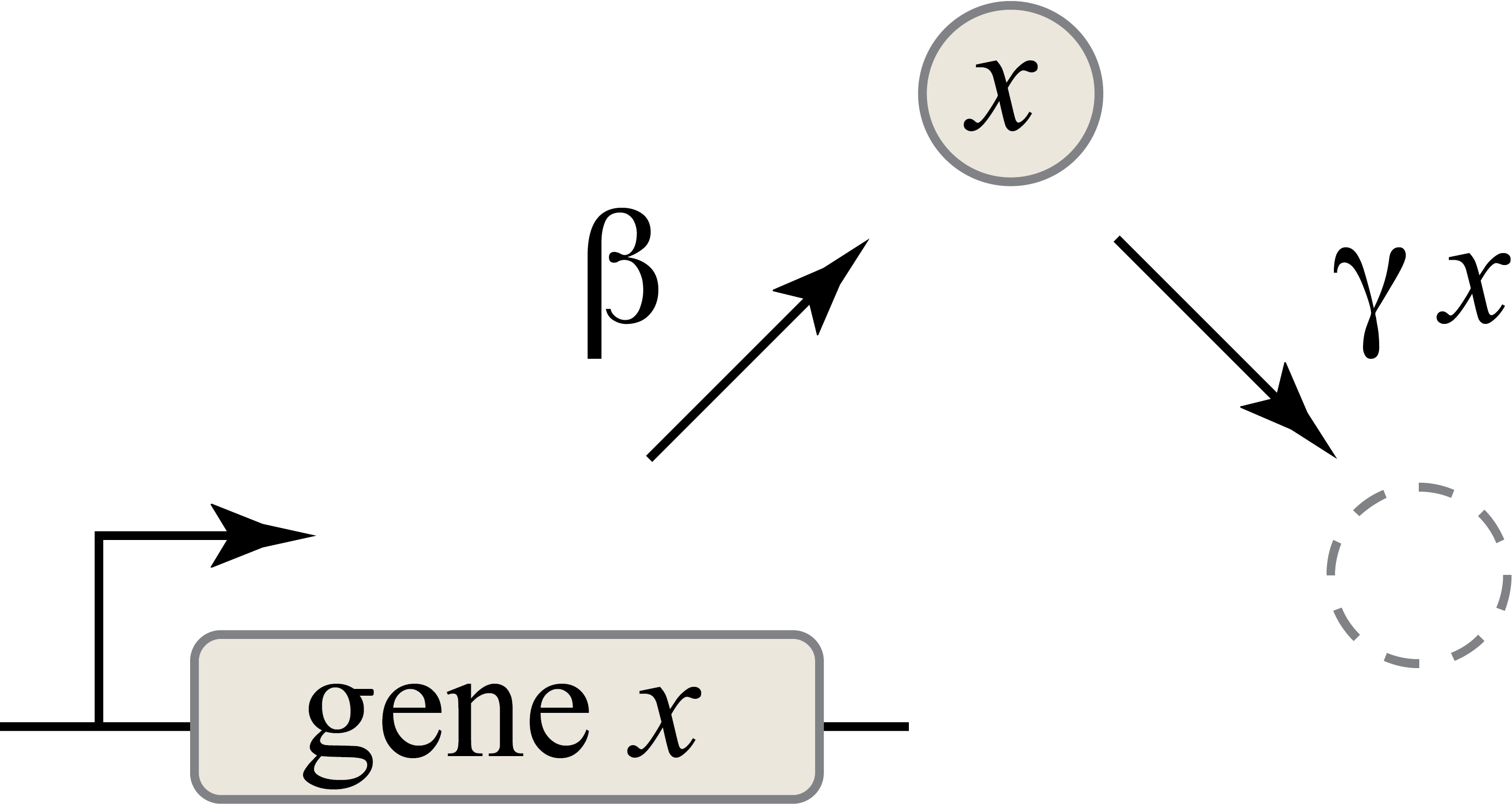
We can then write down a simple ordinary differential equation describing these dynamics:
\begin{align} &\frac{dx}{dt} = \mathrm{production - (degradation+dilution)} \\[1em] &\frac{dx}{dt} = \beta - \gamma x \end{align}
where
\begin{align} \gamma = \gamma_\mathrm{dilution} + \gamma_\mathrm{degradation} \end{align}
A note on effective degradation rates: When cells are growing, protein is removed through both degradation and dilution. For stable proteins, dilution dominates. For very unstable proteins, whose half-life is much smaller than the cell cycle period, dilution may be negligible. In bacteria, mRNA half-lives (1-10 min, typically) are much shorter than protein half-lives. In eukaryotic cells this is not necessarily true. For example, in mammalian cells, mRNA half-lives can be many hours.
Often, one of the first things we would like to know is the concentration of protein under steady state conditions. To obtain this, we set the time derivative to 0, and solve:
\begin{align} &\frac{dx}{dt} = \beta - \gamma x = 0 \\[1em] &\Rightarrow x_\mathrm{ss} = \beta / \gamma \end{align}
In other words, the steady-state protein concentration is proportional to the ratio of production and removal rates. It can be increased either by increasing the production rate or by slowing the removal rate.
Including transcription and translation as separate steps
So far, our description does not distinguish between two key steps in gene expression: transcription and translation. Considering the two processes separately can be important in dynamic and stochastic contexts, including some we will encounter later. To do so, we can simply add an additional variable to represent the mRNA concentration, which is now transcribed, translated to protein, and degraded (and diluted), as shown schematically here:
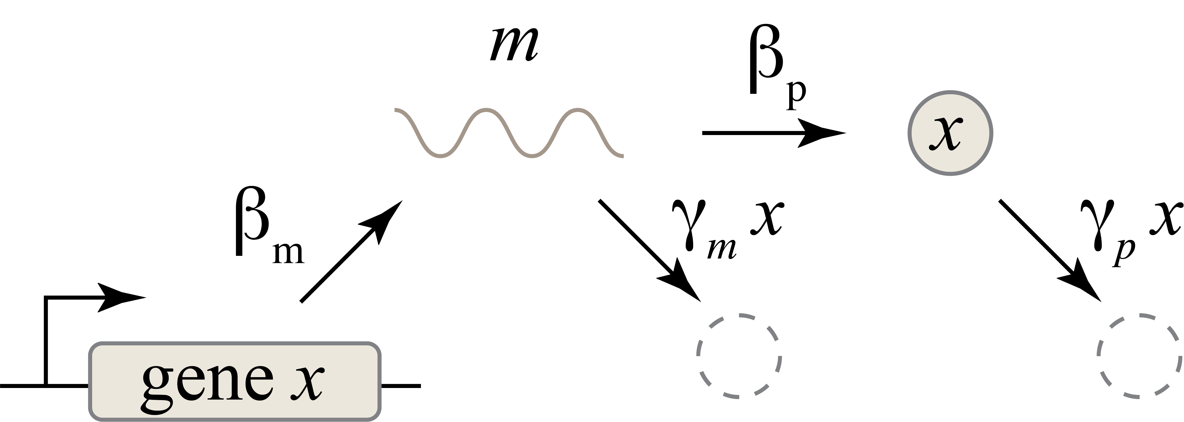
These reactions can be described by two coupled differential equations for the mRNA (\(m\)) and protein (\(x\)) concentrations:
\begin{align} &\frac{dm}{dt} = \beta_m - \gamma_m m, \\[1em] &\frac{dx}{dt} = \beta_p m - \gamma_p x. \end{align}
To determine the steady state mRNA and protein concentrations, we set both time derivatives to 0 and solve. Doing this, we find:
\begin{align} &m_\mathrm{ss} = \beta_m / \gamma_m, \\[1em] &x_\mathrm{ss} = \frac{\beta_p m_\mathrm{ss}}{\gamma_p} = \frac{\beta_p \beta_m}{\gamma_p \gamma_m}. \end{align}
From this, we see that the steady state protein concentration is proportional to the product of the two synthesis rates and inversely proportional to the product of the two degradation rates.
And this gives us our first design question, which you can explore in an end-of-chapter problem: The cell could control protein expression level in at least four different ways. It could modulate any or all of (1) transcription, (2) translation, (3) mRNA degradation, or (4) protein degradation rates, or combinations thereof. Are there tradeoffs between these different options? Are they all used indiscriminately or is one favored in natural contexts?
Repressors enable gene regulation
In principle, genes could be left “on” all the time. In actuality, the cell activity regulates them, turning their expression levels lower or higher depending on environmental conditions and cellular state. Repressors provide a key mechanism for regulation. Repressors are proteins that bind to specific, cognate sequences (binding sites) at or near a promoter, altering its expression. Often the strength of repressor binding depends on external inputs. For example, the LacI repressor normally turns off the genes for lactose utilization in E. coli. However, in the presence of lactose in the media, a modified form of lactose (allolactose) binds to LacI, inhibiting its ability to repress its target genes. (Small molecules that bind to proteins and alter their activities are called allosteric effectors or, in contexts like this, inducers). Thus, in this relatively simple circuit, a nutrient (lactose) regulates expression of the genes that allow its metabolism. (A wonderful book, The lac Operon by Benno Müller-Hill, provides the fascinating scientific and historical saga of this paradigmatic system.)
In the following diagram, we label the repressor R.
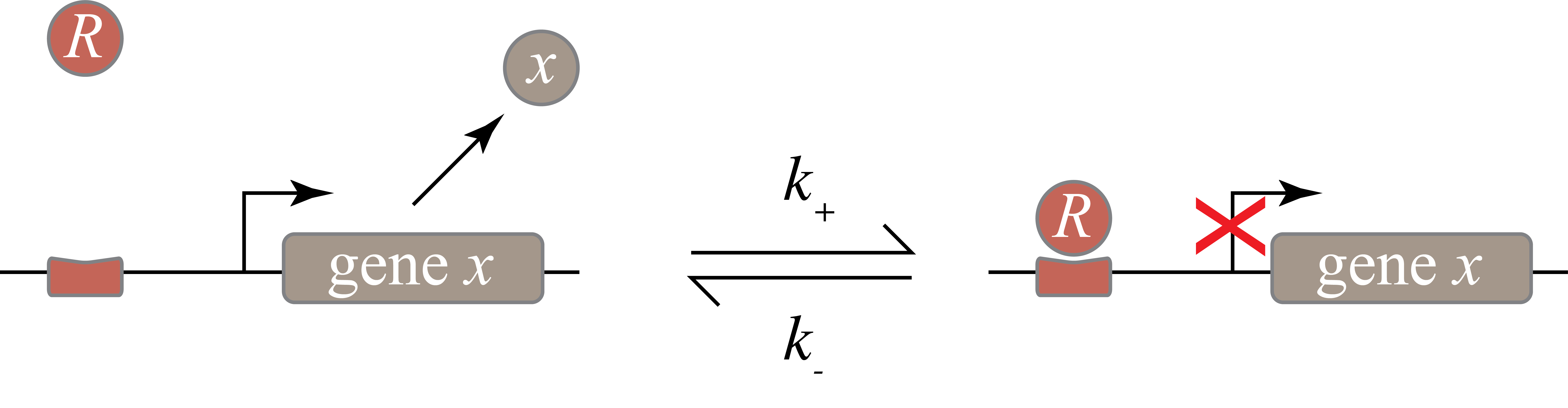
Within the cell, the repressor can bind to, and unbind from, its target site. The expression level of the gene is lower when the repressor is bound and higher when it is unbound. The mean expression level of the gene is then proportional to the fraction of time that the promoter region is not bound with a repressor.
The process of binding and unbinding of a repressor can be represented as the chemical reaction
\begin{align} \require{mhchem} \ce{P + R <=>[k_+][k_-] P}_\mathrm{bound}. \end{align}
We can model the dynamics of this chemical reaction using mass action kinetics in which the rate of a reaction is proportional to the product of the concentrations of its reactants. We therefore represent the “concentration” of target sites in bound or unbound states. Within a single cell an individual site on the DNA is either bound or unbound, but averaged over a population of cells, we can talk about the mean occupancy of the site. Let \(r\) be the concentration of repressor, \(p\) be the concentration of unbound promoter, \(p_\mathrm{bound}\) be the concentration of promoter bound with a repressor. Then,
\begin{align} \frac{\mathrm{d}p}{\mathrm{d}t} = -k_+\,p\,r + k_- p_\mathrm{bound}. \end{align}
We can assume a separation of timescales because both the rates of binding and unbinding of the repressor to the DNA binding site are often fast compared to the timescales over which mRNA and protein concentrations vary. (Note that this assumption is reasonable for many genes in bacteria, but may not apply in other contexts, such as for some mammalian genes.) On the time scale of variation in mRNA and protein concentrations, the repressor-promoter binding-unbinding reaction dynamics are fast and the reaction is essentially at steady state such that \(\mathrm{d}p/\mathrm{d}t \approx 0\), giving
\begin{align} -k_+\,p\,r + k_- p_\mathrm{bound} = 0. \end{align}
If \(p_\mathrm{tot}\) is the total concentration of promoters, bound or not, then \(p_\mathrm{tot} = p + p_\mathrm{bound}\), and we have
\begin{align} -k_+\,p\,r + k_- (p_\mathrm{tot} - p) = 0, \end{align}
which can be rearranged to give the fraction of promoters that are free to allow transcription,
\begin{align} \frac{p}{p_\mathrm{tot}} = \frac{1}{1+r/K_\mathrm{d}}, \end{align}
where we have defined the dissociation constant for repressor-target binding
\begin{align} K_\mathrm{d} = \frac{k_-}{k_+} \end{align}
Because we have a separation of time scales, the rate of production of gene product should be proportional to the probability of the promoter being unbound,
\begin{align} \beta(r) = \beta_0 \frac{p}{p_\mathrm{tot}} = \frac{\beta_0}{1+r/K_\mathrm{d}}. \end{align}
Properties of the simple binding curve
This is our first encounter with a soon to be familiar function. Note that this function has two parameters: \(K_\mathrm{d}\) specifies the concentration of repressor at which the response is reduced to half its maximum value. The coefficient \(\beta_0\) is simply the maximum expression level, and is a parameter that multiples the rest of the function. Also notice that for small values of \(r\), the slope is \(-1/K_d\)
[2]:
# Build theoretical curves for dimensionless r and beta
r = np.linspace(0, 20, 200)
beta = 1 / (1 + r)
init_slope = 1 - r

# Build plot
p = bokeh.plotting.figure(
    frame_height=225,
    frame_width=350,
    x_axis_label="r/Kd",
    y_axis_label="β(r)/β₀",
    x_range=[r[0], r[-1]],
    y_range=[0, 1],
)
p.line(r, init_slope, line_width=2, color="orange", legend_label="initial slope")
p.line(r, beta, line_width=2, legend_label="β(r)/β₀")
p.legend.click_policy = "hide"
p.legend[0].items = p.legend[0].items[::-1]

bokeh.io.show(p)
Gene expression can be “leaky”
In real life, many genes never get repressed all the way to zero expression, even when you add a lot of repressor. Instead, there is a baseline, or “basal”, expression level that still occurs. A simple way to model this is by adding an additional constant term, \(\alpha_0\) to the expression
\begin{align} \beta(R) = \alpha_0 + \beta_0 \frac{p}{p_\mathrm{tot}} = \alpha_0 + \frac{\beta_0}{1+r/K_\mathrm{d}}. \end{align}
Where does such leaky expression come from? Molecular interactions inside a cell are always probabilistic. Repressors are constantly binding and unbinding from their DNA target sites. Even if there are many more repressors than there are genes to repress, there is still typically a finite time interval between the unbinding and the re-binding of a repressor. During these intervals, the competing process of transcription initiation may occur.
Given the ubiquity of leakiness, it is important to check that important circuit behaviors do not require the complete absence of leaky expression.
[3]:
# Build the theoretical curves
r = np.linspace(0, 20, 200)
alpha_0 = .25
beta = alpha_0 + 1 / (1 + r)

# Build plot
p = bokeh.plotting.figure(
    frame_height=225,
    frame_width=350,
    x_axis_label="r/Kd",
    y_axis_label="β(r)/β₀",
    x_range=[r[0], r[-1]],
    y_range=[0, beta.max()],
)
p.line(
    [r[0], r[-1]],
    [alpha_0, alpha_0],
    line_width=2,
    color="orange",
    legend_label="basal (leaky) expression, α₀/β₀",
)
p.line(r, beta, line_width=2, legend_label="β(r)/β₀")
p.legend.click_policy = "hide"
p.legend[0].items = p.legend[0].items[::-1]

bokeh.io.show(p)
Activators enable positive regulation
Genes can be positively regulated by activators as well as negatively regulated by repressors. Treating the case of activation just involves switching the state that is actively expressing from the unbound state to the state where the promoter region is bound by the protein (now called an activator). And, just as small molecule inputs can modulate the binding of a repressor to DNA, so too can they modulate the binding of the activator. In bacteria, one of many examples is the Lux-type quorum sensing system, where the transcription factor LuxR acts as an activator in the presence of its cognate ligand, a signaling molecule produced by cells.
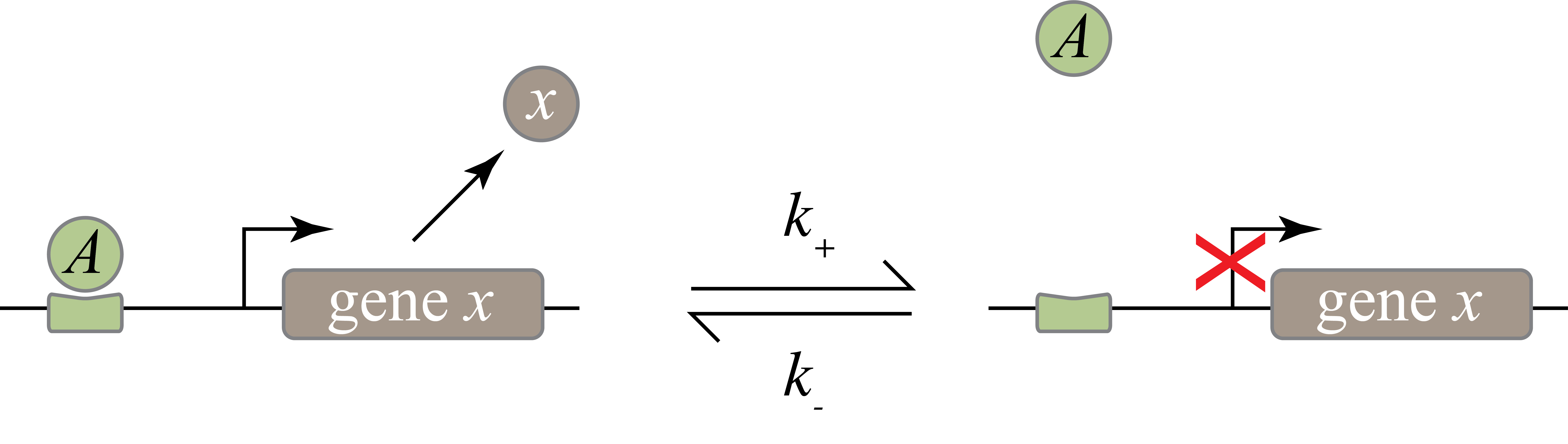
By assuming production in the activator-bound state, we obtain the rate of production of gene product as a function of activator concentration, \(a\):
\begin{align} \beta(a) = \beta_0 \frac{p_\mathrm{bound}}{p_\mathrm{tot}} = \beta_0\,\frac{a/K_\mathrm{d}}{1+a/K_\mathrm{d}}. \end{align}
This produces the opposite, mirror image response compared to repression, shown below with no leakage.
[4]:
a = np.linspace(0, 20, 200)
beta_A = a / (1 + a)
beta_R = 1 / (1 + r)

# Build plot
p = bokeh.plotting.figure(
    frame_height=225,
    frame_width=350,
    x_axis_label="a/Kd, r/Kd",
    y_axis_label="β ∕ β₀",
    x_range=[r[0], r[-1]],
    y_range=[0, 1],
)

p.line(a, beta_A, line_width=2, legend_label="β(a)/β₀")
p.line(r, beta_R, line_width=2, color="tomato", legend_label="β(r)/β₀")
p.legend.location = "center_right"

p.output_backend = 'svg'

bokeh.io.show(p)
Hill functions enable analysis of ultrasensitivity
While the activating and repressing functions we derive above indeed capture the behavior of this simple model of transcriptional regulation, in practice we find that many responses in gene regulation and protein-protein interactions have a more switch-like, or ultrasensitive, shape. Ultrasensitivity can arise from many sources. One important source is cooperativity in molecular interactions. For example, binding of a protein at one DNA binding site can increase the affinity for binding of a second protein at an adjacent site. Or, imagine a protein with an alternative molecular conformation that is stabilized by binding of multiple agonist effector molecules and, in that conformation, has a higher affinity for the same effectors. In these and many other situations, an increasing concentration of one species can have little effect for a while, and then suddenly have a large effect. (See Rob Phillips’s book, The Molecular Switch: Signaling and Allostery for an engaging and rigorous discussion of these mechanisms.)
The Hill function provides a phenomenological way to analyze systems that exhibit ultrasensitive responses. While it can be derived from models of some processes, it is often introduced independently of any specific underlying reaction to analyze how different levels of ultrasensitivity in one process would impact the behavior of the larger circuit.
An activating Hill function is defined by
\begin{align} f_\mathrm{act}(x) &= \frac{x^n}{k^n +x^n} = \frac{(x/k)^n}{1 + (x/k)^n}. \end{align}
The mirror image repressive Hill function is similarly defined as
\begin{align} f_\mathrm{rep}(x) &= \frac{k^n}{k^n +x^n} = \frac{1}{1 + (x/k)^n}. \end{align}
In these expressions, \(k\) represents the concentration at which the function attains half its maximal value and is referred to as the Hill activation constant. It is a measure of the characteristic concentration of \(x\) that is necessary to achieve strong regulation. The Hill coefficient, \(n\), parametrizes how ultrasensitive the response is. When \(n=1\), we recover the simple binding curves introduced above. When \(n>1\), however, we achieve ever sharper, more ultrasensitive, responses. In the limit of \(n=\infty\) the Hill function becomes a perfect step function.
The production rate of the products of genes under control of an activator and repressor, respectively, operating with ultrasensitivity modeled with Hill function is
\begin{align} &\beta(a) = \beta_0\,f_\mathrm{act}(a) = \beta_0 \,\frac{(a/k)^n}{1 + (a/k)^n},\\[1em] &\beta(r) = \beta_0\,f_\mathrm{rep}(r) = \beta_0 \,\frac{1}{1 + (r/k)^n}. \end{align}
Going forward, we will drop the naught subscripts on \(\beta\) (and also on \(\alpha\)) for notational brevity and will write expressions like
\begin{align} &\text{activator-modulated production rate} = \beta \,\frac{(a/k)^n}{1 + (a/k)^n},\\[1em] &\text{repressor-modulated production rate} = \beta \,\frac{1}{1 + (r/k)^n}. \end{align}
To help visualize Hill functions, we plot them below for a various degrees of ultrasensitivity, with activating Hill functions in blue and repressing Hill functions in red.
[5]:
# Values of Hill coefficient
n_vals = [1, 2, 10, 25, np.inf]

# Compute activator response
x = np.concatenate((np.linspace(0, 1, 200), np.linspace(1, 4, 200)))
x_log = np.concatenate((np.logspace(-2, 0, 200), np.logspace(0, 2, 200)))

f_a = []
f_a_log = []
for n in n_vals:
    if n == np.inf:
        f_a.append(np.concatenate((np.zeros(200), np.ones(200))))
        f_a_log.append(f_a[-1])
    else:
        f_a.append(x ** n / (1 + x ** n))
        f_a_log.append(x_log ** n / (1 + x_log ** n))

# Repressor response
f_r = [1 - f for f in f_a]
f_r_log = [1 - f for f in f_a_log]

# Build plots
p_act = bokeh.plotting.figure(
    frame_height=225,
    frame_width=350,
    x_axis_label="x/k",
    y_axis_label="activating Hill function",
    x_range=[x[0], x[-1]],
)
p_rep = bokeh.plotting.figure(
    frame_height=225,
    frame_width=350,
    x_axis_label="x/k",
    y_axis_label="repressing Hill function",
    x_range=[x[0], x[-1]],
)

p_act_log = bokeh.plotting.figure(
    frame_height=225,
    frame_width=350,
    x_axis_label="x/k",
    y_axis_label="activating Hill function",
    x_range=[x_log[0], x_log[-1]],
    x_axis_type="log",
)
p_rep_log = bokeh.plotting.figure(
    frame_height=225,
    frame_width=350,
    x_axis_label="x/k",
    y_axis_label="repressing Hill function",
    x_range=[x_log[0], x_log[-1]],
    x_axis_type="log",
)

# Set up toggling between activating and repressing and log/linear
p_act.visible = True
p_rep.visible = False
p_act_log.visible = False
p_rep_log.visible = False

radio_button_group_ar = bokeh.models.RadioButtonGroup(
    labels=["activating", "repressing"], active=0, width=150
)
radio_button_group_log = bokeh.models.RadioButtonGroup(
    labels=["linear", "log"], active=0, width=100
)

col = bokeh.layouts.column(
    p_act,
    p_rep,
    p_act_log,
    p_rep_log,
    bokeh.models.Spacer(height=10),
    bokeh.layouts.row(
        bokeh.models.Spacer(width=55),
        radio_button_group_ar,
        bokeh.models.Spacer(width=75),
        radio_button_group_log,
    ),
)

radio_button_group_ar.js_on_change(
    "active",
    bokeh.models.CustomJS(
        args=dict(
            radio_button_group_log=radio_button_group_log,
            p_act=p_act,
            p_rep=p_rep,
            p_act_log=p_act_log,
            p_rep_log=p_rep_log,
        ),
        code="""
if (radio_button_group_log.active == 0) {
    if (p_act.visible == true) {
        p_act.visible = false;
        p_rep.visible = true;
    }
    else {
        p_act.visible = true;
        p_rep.visible = false;
    }
}
else {
    if (p_act_log.visible == true) {
        p_act_log.visible = false;
        p_rep_log.visible = true;
    }
    else {
        p_act_log.visible = true;
        p_rep_log.visible = false;
    }
}
""",
    ),
)

radio_button_group_log.js_on_change(
    "active",
    bokeh.models.CustomJS(
        args=dict(
            radio_button_group_ar=radio_button_group_ar,
            p_act=p_act,
            p_rep=p_rep,
            p_act_log=p_act_log,
            p_rep_log=p_rep_log,
        ),
        code="""
if (radio_button_group_ar.active == 0) {
    if (p_act_log.visible == true) {
        p_act_log.visible = false;
        p_act.visible = true;
    }
    else {
        p_act_log.visible = true;
        p_act.visible = false;
    }
}
else {
    if (p_rep_log.visible == true) {
        p_rep_log.visible = false;
        p_rep.visible = true;
    }
    else {
        p_rep_log.visible = true;
        p_rep.visible = false;
    }
}
""",
    ),
)

# Color scheme for plots
colors_act = bokeh.palettes.Blues256[32:-32][:: -192 // (len(n_vals) + 1)]
colors_rep = bokeh.palettes.Reds256[32:-32][:: -192 // (len(n_vals) + 1)]

# Populate glyphs
for i, n in enumerate(n_vals):
    legend_label = "n → ∞" if n == np.inf else f"n = {n}"
    p_act.line(x, f_a[i], line_width=2, color=colors_act[i], legend_label=legend_label)
    p_rep.line(x, f_r[i], line_width=2, color=colors_rep[i], legend_label=legend_label)
    p_act_log.line(
        x_log, f_a_log[i], line_width=2, color=colors_act[i], legend_label=legend_label
    )
    p_rep_log.line(
        x_log, f_r_log[i], line_width=2, color=colors_rep[i], legend_label=legend_label
    )

# Reposition legends
p_act.legend.location = "bottom_right"
p_act_log.legend.location = "bottom_right"

bokeh.io.show(col)
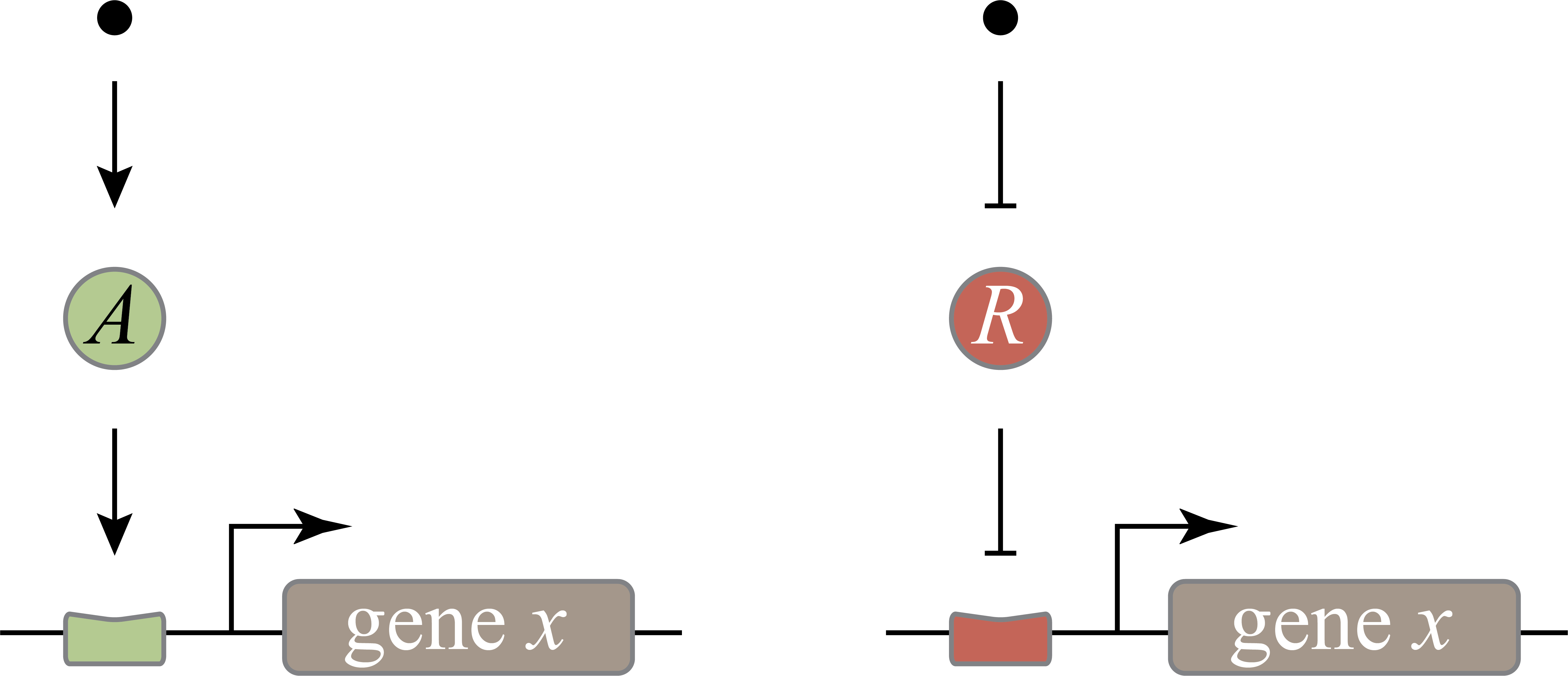
When should a circuit use an activator and when should it use a repressor?
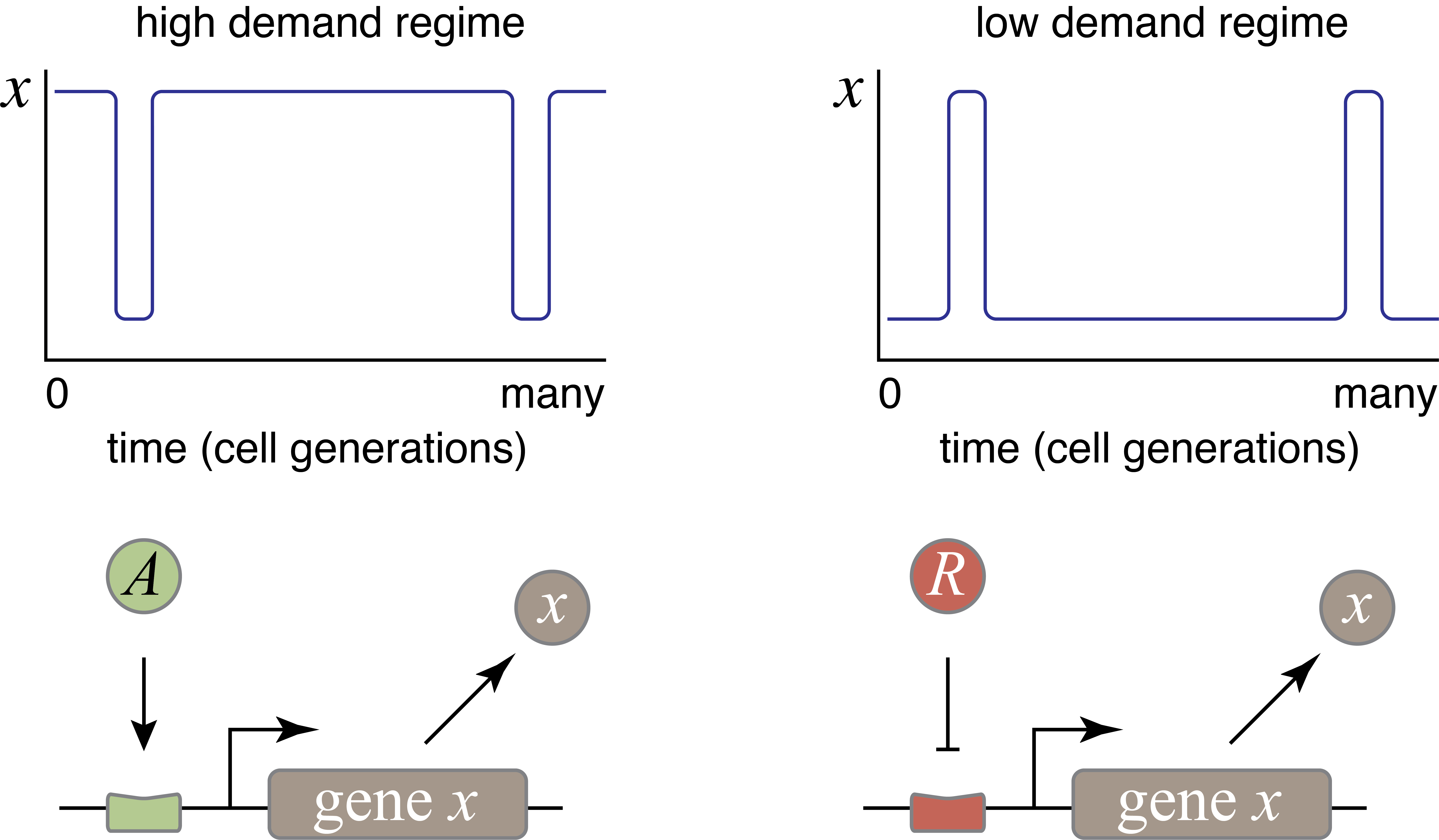
*And now at least we have reached a true design puzzle: We could design gene regulation systems that turn on in the presence of a specific molecular signal (we will call this the inducer) in two, seemingly equivalent, ways. The gene could be regulated by an activator whose activity is turned on by the inducer (see left figure below), or alternatively, it could be regulated by a repressor whose activity is inhibited by the inducer (see right figure below).
Which should it choose? Are they completely equivalent? Or is there a reason to prefer one mode or another in any given context? How could we know? Which would you choose if you were designing a synthetic circuit of this type?
Michael Savageau posed this question in the context of bacterial metabolic gene regulation (Savageau, 1977). He identified “demand” for a gene product as a critical factor that influences the choice of activation or repression. Demand can be defined as the fraction of time that the gene is needed at the high end of its expression range in the cells natural environments. Savageau made the empirical observation that high-demand genes are more frequently regulated by activators, while low-demand genes are more often regulated by repressors.
Savageau suggested that this relationship could be explained by a “use it or lose it” rule of evolutionary selection. In bacteria, mutations appear frequently enough (\(10^{-10}\) - \(10^{-9}\) per bp per replication cycle) that virtually any mutation is present within a colony. Under these conditions, a regulatory system that is unnecessary would not be retained by selection. A high demand gene controlled by an activator requires the activator to be expressed most of the time. Under these conditions, he argued, evolution would select against mutations that eliminate the activator. By contrast, if the same high demand system were regulated by a repressor, then most of the time, there would be weaker selection against mutations that removed the repressor, increasing the potential for evolutionary loss of the regulatory system. This reasoning assumes no direct fitness advantage for either regulation mode, just a difference in the average strength of selection pressure needed to maintain the two systems, and qualitatively agrees with the observed correlation between demand type of regulation.
In 2009, Gerland and Hwa formulated and analyzed a mathematical model to explore how the demand rule depends on population size and the temporal durations of the low and high demand environments. They showed that the “use it or lose it” principle indeed dominates when timescales of switching between low and high demand environments are long, and populations are small. However, they also pointed out that the opposite, more intuitive, demand rule (which they term “wear and tear”) could be selected in other regimes, when accumulated mutations in the regulatory system diminish the function for the more prevalent behavior.
In between, Shinar, et al. introduced a completely different explanation for the demand rule. They noted that transcription factors are never perfectly specific for their cognate DNA binding sites. Rather, they bind to non-specific DNA sites with lower, but non-zero, affinities. While individually weak, the effects of many such non-specific interactions could, collectively, be significant. They therefore suggested that “naked” DNA binding sites not bound to proteins are intrinsically more susceptible to inappropriate, non-specific binding of other transcription factors, potentially leading to erroneous gene expression. These expression “errors” impose non-zero fitness cost. Cells can minimize that cost by keeping sites occupied most of the time.
This explanation make the same qualitative predictions as Savageau’s explanation but for different reasons. Here, a high demand gene should preferentially use an activator since this arrangement minimizes unoccupied binding sites more of the time. Conversely, a low demand gene would preferentially use repression to maintain the binding site in a bound state under most conditions. This argument can be generalized to other examples of seemingly equivalent regulatory systems and is described in Alon’s Introduction to Systems Biology.
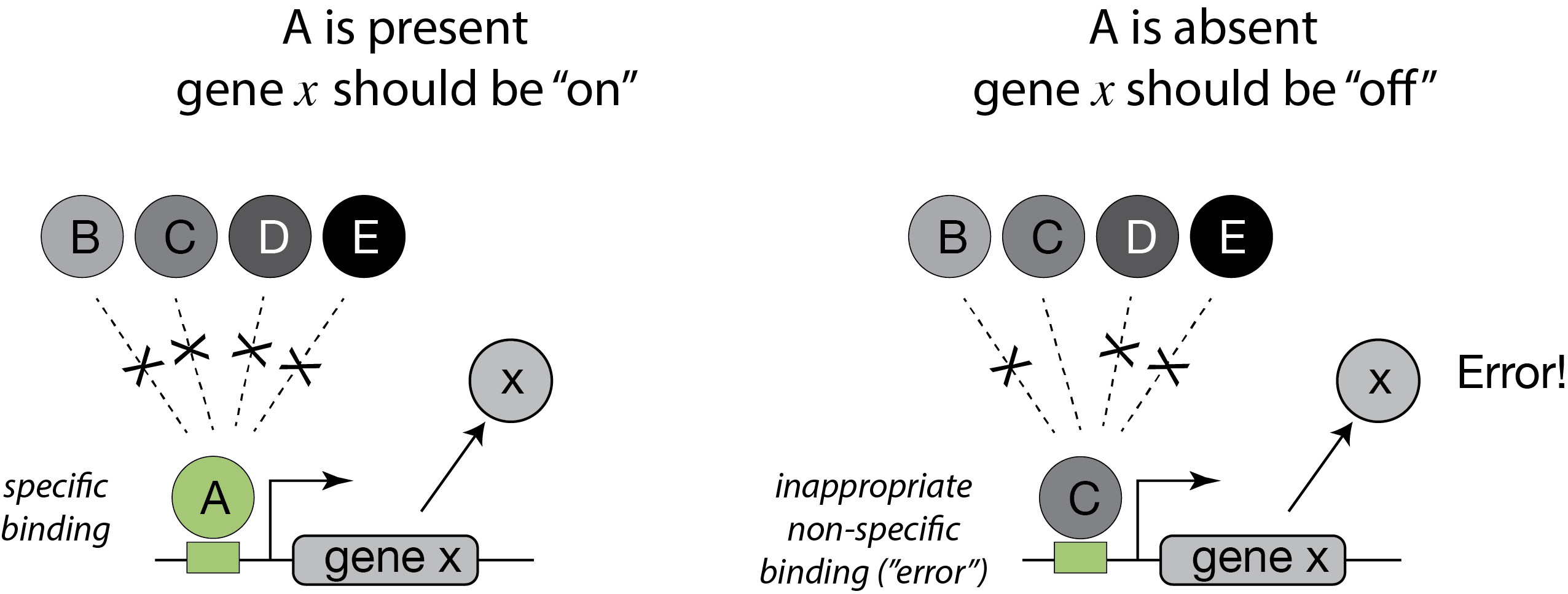
In this figure, an activator, denoted A binds strongly and specifically to its target site. In the absence of the activator, that site could also be bound non-specifically, and inappropriately by a range of other factors, denoted B-E.
Remarkably, despite all of this beautiful work, we still lack definitive experimental evidence to fully resolve this fundamental design question. As a challenge in the end-of-chapter problems, you are aked to devise an experimental way to discriminate among these potential explanations.
References
Alon, U., An Introduction to Systems Biology: Design Principles of Biological Circuits, 2nd Ed., Chapman and Hall/CRC, 2019. (link)
Gerland, U. and Hwa, T., Evolutionary selection between alternative modes of gene regulation, Proc. Natl. Acad. Sci. USA, 106, 8841–8846, 2009. (link)
Gunawardena, J., Models in biology: ‘accurate descriptions of our pathetic thinking’, BMC Biology, 12, 29, 2014. (link)
Hanahan, D. and Weinberg, R. A., The hallmarks of cancer, Cell, 100, 57–70, 2000. (link)
Horowitz, P. and Hill, W., The Art of Electronics, 3rd. Ed., Cambridge University Press, 2015. (link)
Jacob, F. and Monod, J., On the regulation of gene activity, Cold Spring Harb. Symp. Quant. Biol., 26, 193–211, 1961. (link)
Judson, H. F., The Eighth Day of Creation: The Makers of the Revolution in Biology, Commemorative Ed., Cold Spring Harbor Laboratory Press, 1996. (link)
Müller-Hill, B., The lac Operon: A Short History of a Genetic Paradigm, De Gruyter, 1996. (link)
Phillips, The Molecular Switch: Signaling and Allostery, Princeton University Press, 2020. (link)
Savageau, M. A., Design of molecular control mechanisms and the demand for gene expression, Proc. Natl. Acad. Sci. USA, 74, 5647–5651, 1977. (link)
Shinar, G., et al., Rules for biological regulation based on error minimization, Proc. Natl. Acad. Sci. USA, 103, 3999–4004, 2006. (link)
Problems
Computing environment
[6]:
%load_ext watermark
%watermark -v -p numpy,bokeh,jupyterlab
Python implementation: CPython
Python version       : 3.10.10
IPython version      : 8.10.0

numpy     : 1.23.5
bokeh     : 3.1.0
jupyterlab: 3.5.3