15. The noisy, noisy nature of gene expression: How stochastic fluctuations create variation

---

Concepts

• Intrinsic and extrinsic noise

Techniques

• Plug-in estimates

• Pairs bootstrap

• Generative Bayesian modeling

---

# Colab setup ------------------
import os, sys
if "google.colab" in sys.modules:
    data_path = "https://biocircuits.github.io/chapters/data/"
else:
    data_path = "data/"
# ------------------------------

import numpy as np
import pandas as pd

import bokeh.models
import bokeh.plotting
import bokeh.io

bokeh.io.output_notebook()

Loading BokehJS ...

---

So far, for the most part, we have treated circuits in the cell as if they are continuous and deterministic. We have written systems of ordinary differential equations to describe the dynamics of mRNA and protein concentrations in cells. This framework ignores the discreteness of molecules, and the stochastic (intrinsically random) nature of molecular interactions. It would be a perfectly reasonable approximation if cells were macroscopic systems with very large numbers of copies of each molecular species. However, most living cells are not macroscopic. They are small — a bacterial cell has a volume of a femtoliter (\(10^{-15}\) liters). Small size has consequences. Unpredictable fluctuations in the number of copies of a protein—biological “noise”—can dramatically affect the behavior of the cell. To detect, quantify, and model systems with noise, we will need new experimental, computational, and mathematical approaches.

Over the next chapters we will focus on understanding the sources and dynamics of noise, methods to analyze noise, and the potentially useful functional roles of noise in biological systems. To do so, we will use the mathematical machinery of probability, which is an essential tool for diverse problems in biology.

Noise is present in genetic circuits, and cells are like burritos

One cell may seem at first glance identical to any other cell living alongside it in the same conditions. However, if we could somehow look inside each cell, and observe the various molecular species populating each cell, we would notice dramatic variations from cell to cell. In part, this is because the number of copies of many proteins and mRNA molecules in the cell are small. Wi and coworkers (Cell, 2014) used ribosome profiling to obtain estimates for absolute protein counts of various transcription factors in bacteria. They found that half of repressors have copy numbers below 100 per genome equivalent and 90% of activators do as well. About 10% of repressors and 50% of activators have copy numbers of 10 or below. These numbers are small, difficult for the cell to control precisely, and therefore susceptible to fluctuations.

Roughly speaking, we can call random deviations from what we might expect in a deterministic view of gene expression stochasticity, or noise. Nearly all cellular processes are susceptible to noise for a host of reasons, especially low copy numbers of molecular regulators of gene expression. We will provide a more careful definition of noise momentarily.

But first, consider the “model” of an E. coli cell depicted below. From the outside (left image), it appears as a simple rod-shaped object, encapsulating what one might incorrectly assume is a homogeneous well-mixed continuum of biochemical mush inside. However, if we were to slice open the cell (right image), the low copy numbers of certain molecules and their spatial heterogenetiy become apparent. Within each cell, the copy numbers and locations of different molecules can vary dramatically over time, just as they vary from cell to cell. Like burritos, no two cells are completely identical. (Unlike this burrito, most bacteria lack cheese in their periplasm.)

Early approaches to detecting and quantifying cellular variation

An early non-cellular demonstration of how fluctuations in molecule numbers between cells could produce large fluctuations in molecular states was performed by Boris Rotman (PNAS, 1961). Seeking to test whether individual enzyme molecules had identical activities, he diluted β-D-galactosidase down in liquid droplets, with a mean concentration of ~1 molecule per droplet and then assayed their activitity in each droplet. The activity measurement used a fluorescent substrate 6HFP, which glows green when it is cleaved by β-D-galactosidase.

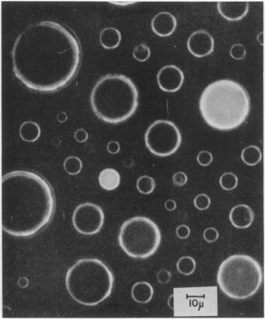
Drops showed quantized activities proportional to the number of enzyme copies in the droplet. Looking at the drops, the heterogeneity in cleaved substrate is striking. It vividly demonstrates how the regime of low copy numbers of molecules produce variable responses. But this is just an inaminate droplet. Do analogous sources of variation occur in living cells?

Stepping back a few years, in 1945, Max Delbrück sought to quantify the origins of heterogenity in a biological process—the infection of E. coli by phages. He measured the number of new phage particles produced when a single phage infected an individual cell. The distribution of this “burst size” was broad, spanning a range from 20 to more than 1000. If phage infection were a deterministic process, and phage particles were identical, and E. coli cells were similar to one another, then why would different infection events produce such wildly different outcomes? Clearly, at least one of these assumptions must be false. But mid-twentieth century tools did not allow one to identify the source of this variation.

Later, in 1998, Arkin, Ross, and McAdams stochastically simulated lambda phage development, and showed that, at least in principle, stochastic noise in the phage infection process, could be sufficient to control the outcome of the decision between lysis and lysogeny after an infection.

A major leap in our understanding of how variation originates occurred in 1994, when the gene coding for the green fluorescent protein of Aequorea victoria jellyfish was cloned and expressed in other organisms by Martin Chalfie and colleagues. Suddenly it became possible to follow gene expression in individual living cells. Discoveries that were previously impossible now became inevitable, and nowhere more so than in the study of noise. Green fluorescent protein and a growing palette of multi-colored derivatives revealed heterogeneity directly. For example, in the image below, we see individual E. coli cells, each expressing yellow fluorescent protein (YFP) under control of the LacI promoter. Although these cells come from a clonal population, they vary vary dramatically in their fluoescent intensity. This provides a direct view of heterogeneity in the expression of a single gene.

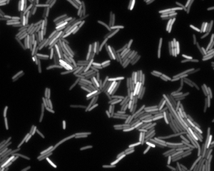
This sort of gene expression heterogeneity is ubiquitous across diverse cellular systems, including bacteria, yeast, and mammals. Even within a multinucleate muscle cell, different nuclei can show different expression levels of the same gene.

But we have to be careful. Heterogeneity could arise in many ways, not all of which we would consider biological “noise.” For example, different cells might find themselves in slightly different environments, encountering different concentrations of signaling molecules. Even if they were behaving deterministically, these differences could activate different gene expression responses or other cellular behaviors. By biological noise, we have in mind stochastic processes operating within the cell that would continue to generate heterogeneity, even if environmental conditions could somehow be held perfectly constant.

Two colors allow analysis of stochastic noise in gene expression

Consider the following thought experiment: Imagine a population of exactly identical cells, all placed in identical environments. A little while later, we check back on these cells and see what has happened to them. If cellular behavior is deterministic, then the cells might have changed—grown longer, for example, or added a few flagella—but they would have all changed in precisely the same way and therefore remained identical to one another. On the other hand, stochasticity, or noise, could cause the properties of these cells to diverge over time. For instance, a stochastic fluctuation in the concentration of a transcription factor in one cell could activate genes that would not be activated in another cell. Thus, if we could prepare two cells in identical states, place them in identical environments, and then monitor them over time, we could detect the effects of noise on their development.

This is an appealing conceptual way to define noise, but infeasible experimentally. The problem is that there is no way to prepare two cells in the same state. Even two sister cells—as closely related as cells can be—show clear observable differences in size, shape, and other properties.

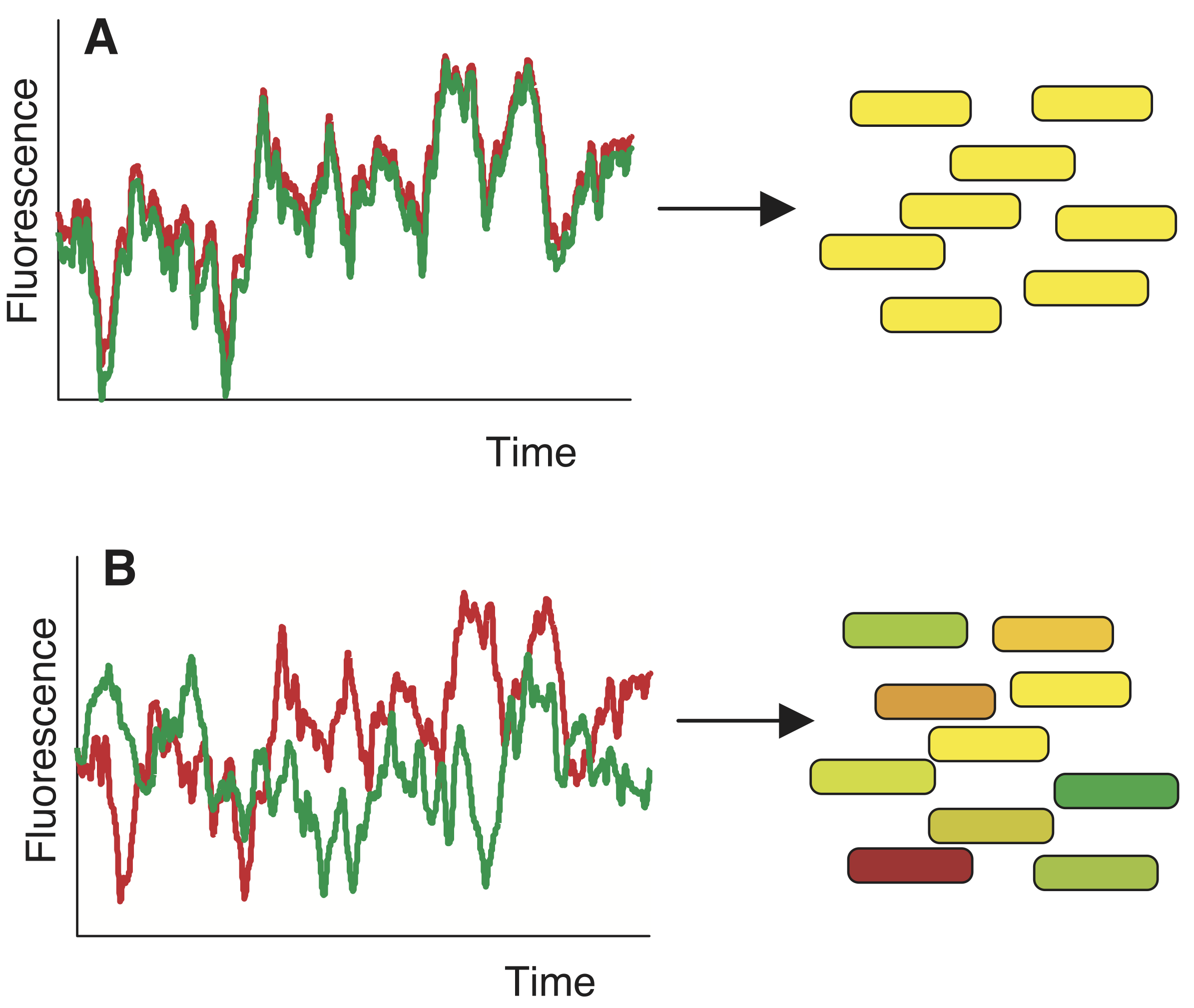
While we cannot put two identical cells in the same environment, we can put two (nearly) identical genes in the same cell. This is conceptually related, and allows us to think of these two genes as two independent stochastic samples of the same underlying process. If gene expression is a deterministic process that is influenced by the state of the cell, then both copies of the gene should “feel” the same intracellular environment and behave identically over time, as in panel A of the image below. Some cells may be more efficient at transcribing or translating genes, but that condition should effect both colors similarly. On the other hand, if the process of transcription or translation is noisy, then expression of each gene could fluctuate independently, producing very different levels of the two proteins in the same cell, as in panel B.

To perform this experiment, Elowitz et al developed a system in which identical promoters were used to express two distinguishable fluorescent proteins of different colors, cyan (CFP) and yellow (YFP). These two genes are nearly identical, differing only in a few point mutations. The authors were careful to integrate the two genes at opposite points in the chromosome, equidistant from the origin of replication, to maintain similar mean gene copy numbers. They also verified that the overall fluorescence distributions across the cell population were statistically indistinguishable, as long as the fluorescence units of one cell were rescaled to match those of the other.

A typical result is shown in the images below.

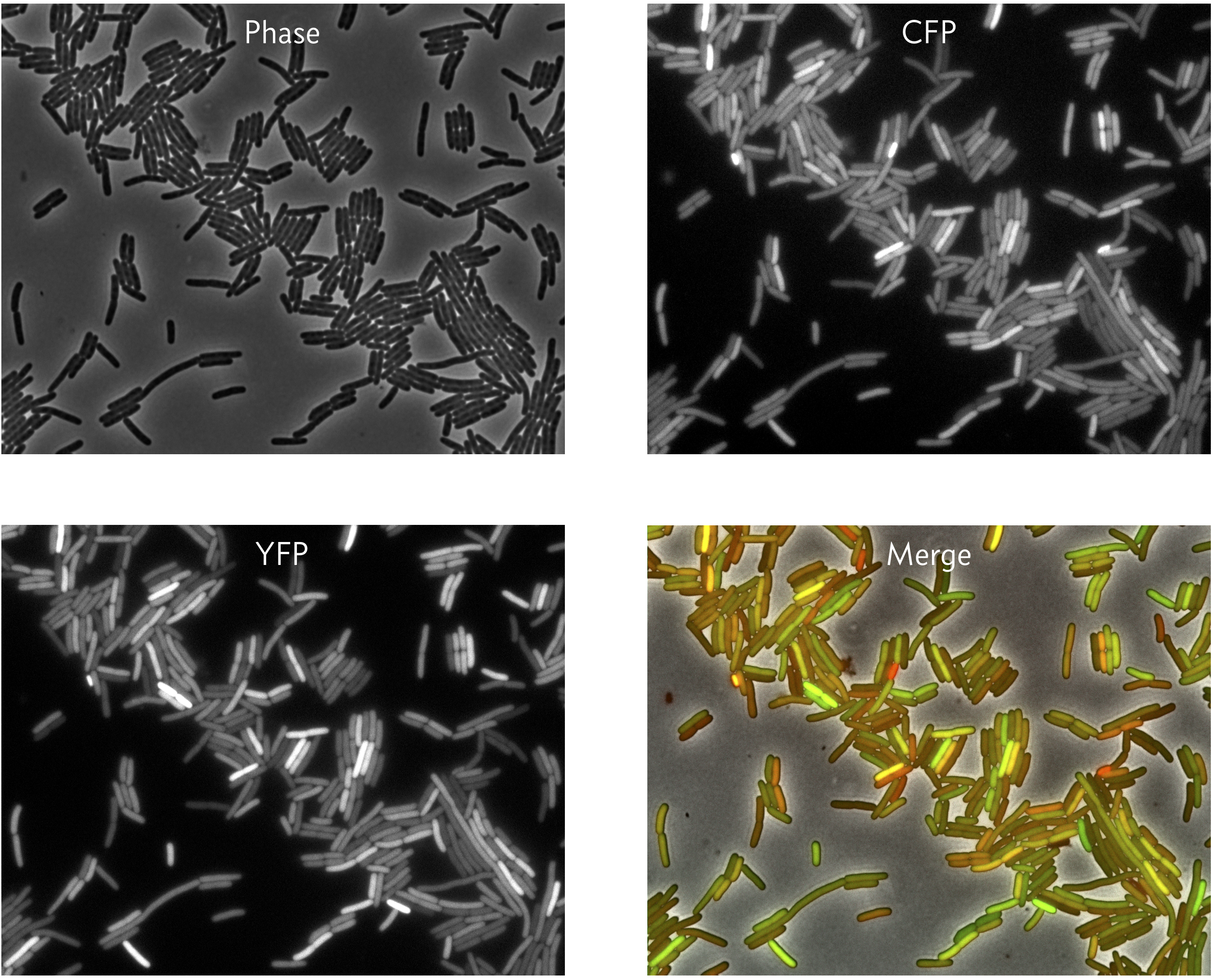
We can see that in some cells, both the CFP and YFP levels are high (yellow in the merge), but in other cases, the CFP and YFP levels differ in expression (green or red in the merge). These images reveal that two genes can show at least partly independent variation in expression. In a sense, they are portraits of noise.

The rest of this chapter addresses how measurements like these can be used to discriminate and measure different sources of noise.

Two flavors of noise: intrinsic and extrinsic

Now that we have a framework for experimentally analyzing gene expression noise, we can think more carefully about how to define it.

Consider one gene product of interest in these cells (such as YFP in the image above). We can define the total noise, \(\eta_\mathrm{tot}\), as the coefficient of variation of the copy numbers of the gene product. The coefficient of variation is the standard deviation of the copy number divided by the mean copy number, or

\begin{align} \eta_\mathrm{tot}^2 = \frac{\left\langle n^2\right\rangle - \left\langle n\right\rangle ^2}{\left\langle n\right\rangle ^2}, \end{align}

where \(n\) is the copy number and where \(\langle n \rangle\) denotes the expectation value of \(n\). If the standard deviation is smaller than the mean, as we would expect in the case of systems with large molecule copy numbers, we have low noise. By contrast, if the standard deviation is large compared to the mean, as occurs in smaller systems, noise typically grows. The coefficient of variation is thus a natural way to measure variation.

How could these variations in gene expression come about? Fluctuations in the concentrations of polymerases or ribosomes within the cell, or variations in the cellular environment, would all be expected to generated variation in the expression level of both of the genes. We define them as upstream of, or extrinsic to, the gene itself.

On the other hand, we might also have fluctuations in gene expression due to the inherent stochasticity of the gene expression process itself. For example, within any given time interval, transcription initiation might occur or not at a given gene depending on whether polymerase happens to bind to the promoter and productively initiate transcription. These types of noise represent intrinsic noise. More precisely,

• Intrinsic noise results from stochastic effects in the processes of transcription and translation that occur independently at each copy of the gene. These effects lead to fluctuations in \(n(t)\). The fluctuations in the copy number of the protein of interest are due to fluctuations that affect only the gene of interest. Operationally, intrinsic noise leads to uncorrelated variation in two identical genes in the same cellular environment. Intrinsic noise fundamentally limits the precision of regulation.

• Extrinsic noise results from “upstream” variations in other molecular species, such as RNA polymerase, ribosomes, and chemical species in the cell’s environment. These factors vary over time and can impact the expression level of both copies of the gene of interest, producing correlated variation in the expression of all target genes they affect.

An important realization is that the terms intrinsic and extrinsic are defined relative to a particular system. If the system is a single gene, then variation in the ribosome concentration is an extrinsic feature. On the other hand, if the system of interest is enlarged to include the whole cell, then those same fluctuations could be regarded as intrinsic.

A second important point is that noise propagates. Ribosomes are composed of RNA and protein products of genes. If their expresion is intrinsically noisy, it could lead to variations in ribosome levels. Those variations would act as extrinsic noise sources for a typical gene. In this way, noise is continually generated, propagated, and transformed within the cell.

Segmentation and scaling of fluorescence

We will now consider the problem of experimentally quantifying noise from the two-color experiment images, like those above. First, the images must be segmented, which means that each pixel in the image needs to be labeled with a unique number corresponding to which bacterium (or background) it belongs. The phase contrast image is used for this purpose to avoid segmenting on the same signal you are trying to measure. Next, the intensities of the pixels in each channel (CFP and YFP) for each bacterium are summed to give a total intensity. The integrated CFP intensity for cell \(i\) is

\begin{align} c_i = c_0 n_{c,i}, \end{align}

where \(n_{c,i}\) is the copy number of CFP in cell \(i\). The constant \(c_0\) is determined by the fluorescent yield of YFP, microscope settings, etc. Similarly, the integrated YFP intensity for cell \(i\) is

\begin{align} y_i = y_0 n_{y,i}. \end{align}

It is in general very difficult to measure \(c_0\) or \(y_0\). While we could have more sophisticated statistical models to try to ascertain them, we will instead scale the YFP intensity in our image processing such that

\begin{align} \langle y \rangle = \langle c \rangle. \end{align}

The assumption in doing so is that the mean copy number of YFP and CFP are equal. This is an important assumption, which hopefully holds because of the careful construction of the promoters on the chromosome, and is one we will rely on going forward.

Do do the scaling in practice, if \(\{c_i, y_i\}\) is the set of \(N\) cellular CFP and YFP integrated intensities we measured and

\begin{align} \bar{c} = \frac{1}{N}\sum_{i=1}^N c_i, \\[1em] \bar{y} = \frac{1}{N}\sum_{i=1}^N y_i \end{align}

are the arithmetic mean of the CFP and YFP intensities, we adjust

\begin{align} c_i \leftarrow c_i / \bar{c},\\[1em] y_i \leftarrow y_i / \bar{y}, \end{align}

which enforces that the means are equal (and both arbitrarily equal to one). With these rescaled intensities, the prefactors connecting the fluorescent intensity to copy number are equal, or \(c_0 = y_0\).

Plug-in estimates for intrinsic, extrinsic, and total noise

As our first approach to estimating the intrinsic and extrinsic noise from our data set \(\{c_i, y_i\}\), let us assume that we do not know the probability distribution describing \(\{c_i, y_i\}\). Since we do not know the distribution, we will resort to making plug-in estimates of the moments of the distribution to estimate quantities such as \(\langle n^2 \rangle\). Remember that going forward, we assume that the data have already been properly scaled to have the same mean.

To compute the total noise, we need to compute the variance in gene expression. Since both CFP and YFP are on identical promoters, we can group them together as a single species in this calculation. The plug-in estimate for the total variance is then

\begin{align} V_\mathrm{tot} = \frac{1}{2N}\sum_{i=1}^N\left[\left(c_i - \bar{c}\right)^2 + \left(y_i - \bar{y}\right)^2\right] = \frac{1}{2}\left(\overline{c^2} - \bar{c}^2 + \overline{y^2} - \bar{y}^2\right). \end{align}

The factor in the denominator is \(2N\) because we have two fluorescent species in each cell.

The intrinsic noise comes from within-cell variation. This is quantified by the difference in fluorescence between the CFP and YFP fluorescence in each cell. This variation is quantified by the mean-square difference,

\begin{align} V_\mathrm{int} = \frac{1}{2N}\sum_{i=1}^N\left(c_i - y_i\right)^2 = \frac{1}{2}\left(\overline{c^2} + \overline{y^2}\right) - \overline{cy}. \end{align}

Note that we again divide by two because both the CFP and YFP expression are subjected to the same intrinsic noise. Since \(V_\mathrm{int}\) accounts for the intrinsic variance, we define the remainder of the variance to be due to extrinsic noise,

\begin{align} V_\mathrm{ext} = V_\mathrm{tot} - V_\mathrm{int} = \overline{cy} - \frac{1}{2}\left(\bar{c}^2 + \bar{y}^2\right) = \overline{cy} - \bar{c}\bar{y}, \end{align}

where in the last equality we have used the fact that \(\bar{c} = \bar{y}\). We recognize that the extrinsic noise is given by the plug-in estimate for the covariance. We can now write expressions for the plug-in estimates for the noise by dividing these variances by the square of the mean expression, \(\bar{c}\bar{y}\) (again, because \(\bar{c} = \bar{y}\)).

\begin{align} &\eta_\mathrm{tot}^2 = \frac{V_\mathrm{tot}}{\bar{c}\bar{y}} = \frac{1}{2\bar{c}\bar{y}}\left(\overline{c^2} - \bar{c}^2 + \overline{y^2} - \bar{y}^2\right),\\[1em] &\eta_\mathrm{int}^2 = \frac{V_\mathrm{int}}{\bar{c}\bar{y}} = \frac{1}{2\bar{c}\bar{y}}\left(\overline{c^2} + \overline{y^2}\right) - \overline{cy}\\[1em] &\eta_\mathrm{ext}^2 = \frac{V_\mathrm{ext}}{\bar{c}\bar{y}} = \frac{\overline{cy} - \bar{c}\bar{y}}{\bar{c}\bar{y}}. \end{align}

Computing the intrinsic and extrinsic noise from experimental data

As an example, let us compute the intrinsic and extrinsic noise from experimental data. We will consider two data sets from the Elowitz, et al. paper, both of which are contained in this CSV file. One set of measurements is for the M22 strain, which has the CFP/YFP under control of LacI setup in E. coli we have previously described. The other set of measurements is for the D22 strain, which has a deletion of the recA gene, which is responsible for rescuing stalled replication forks.

Let’s plot the two data sets and compare.

# Read in the data set
df = pd.read_csv(os.path.join(data_path, "elowitz_et_al_2002_fig_3a.csv"))

# Extract measurements into Numpy arrays
m22_cfp = df.loc[
    (df["strain"] == "m22") & (df["fluorophore"] == "cfp"), "intensity"
].values
m22_yfp = df.loc[
    (df["strain"] == "m22") & (df["fluorophore"] == "yfp"), "intensity"
].values
d22_cfp = df.loc[
    (df["strain"] == "d22") & (df["fluorophore"] == "cfp"), "intensity"
].values
d22_yfp = df.loc[
    (df["strain"] == "d22") & (df["fluorophore"] == "yfp"), "intensity"
].values

# Scale the measurements by their means
m22_cfp /= m22_cfp.mean()
m22_yfp /= m22_yfp.mean()
d22_cfp /= d22_cfp.mean()
d22_yfp /= d22_yfp.mean()

# Generate plot
p = bokeh.plotting.figure(
    frame_width=250,
    frame_height=250,
    x_axis_label="CFP",
    y_axis_label="YFP",
    x_range=[0.675, 1.4],
    y_range=[0.675, 1.4],
)
p.circle(m22_cfp, m22_yfp, alpha=0.3, legend_label="M22")
p.circle(d22_cfp, d22_yfp, color="orange", alpha=0.3, legend_label="D22")
p.legend.location = "bottom_right"
p.legend.click_policy = "hide"
p.legend.background_fill_alpha = 0.7

bokeh.io.show(p)

The apparent positive covariance is indicative of the presence of extrinsic noise. We will now proceed to compute plug-in estimates for the intrinsic, extrinsic, and total noise.

def plugin_noise(c, y):
    """Plug-in estimates for noise"""
    Vtot = np.var(np.concatenate((c, y)), ddof=0)
    Vext = np.cov(c, y, ddof=0)[0, 1]
    Vint = Vtot - Vext

    return np.sqrt(np.array([Vint, Vext, Vtot]) / c.mean() / y.mean())


# Compute plug-in estimates
m22_noise = plugin_noise(m22_cfp, m22_yfp)
d22_noise = plugin_noise(d22_cfp, d22_yfp)

# Print the result
print(
    """
M22
---
intrinsic: {0:.4f}
extrincic: {1:.4f}
total:     {2:.4f}

D22
---
intrinsic: {3:.4f}
extrincic: {4:.4f}
total:     {5:.4f}
""".format(
        *m22_noise, *d22_noise
    )
)

M22
---
intrinsic: 0.0554
extrincic: 0.0540
total:     0.0774

D22
---
intrinsic: 0.0814
extrincic: 0.0809
total:     0.1147

We can compute confidence intervals on these values using pairs bootstrap.

# Random number generator for resampling
rng = np.random.default_rng()

# Function to draw a pairs bootstrap replicate
def draw_bs_rep(c, y):
    bs_inds = rng.choice(np.arange(len(c)), len(c))
    bs_c, bs_y = c[bs_inds], y[bs_inds]
    return plugin_noise(bs_c, bs_y)


# Generate bootstrap replicates
n_reps = 100000
m22_reps = np.array([draw_bs_rep(m22_cfp, m22_yfp) for _ in range(n_reps)])
d22_reps = np.array([draw_bs_rep(d22_cfp, d22_yfp) for _ in range(n_reps)])

# Compute 95% confidence interval
m22_confint = np.percentile(m22_reps, [2.5, 97.5], axis=0)
d22_confint = np.percentile(d22_reps, [2.5, 97.5], axis=0)

Now that we have the confidence intervals, we can plot our estimates for the noise with the 95% confidence interval.

# Organize results for convenient plotting
noises = ["intrinsic", "extrinsic", "total"]
strains = ["M22", "D22"]
noise = [m22_noise, d22_noise]
confint = [m22_confint.T, d22_confint.T]
data = [
    ((s, n), confint[i][j, 0], confint[i][j, 1], noise[i][j])
    for i, s in enumerate(strains)
    for j, n in enumerate(noises)
]
df_noise = pd.DataFrame(
    columns=["strain_noise", "2.5", "97.5", "plugin"], data=data
)

# Build data source and factor range for plot
y_range = bokeh.models.FactorRange(*df_noise["strain_noise"][::-1])
source = bokeh.models.ColumnDataSource(df_noise)

# Build the plot
p = bokeh.plotting.figure(y_range=y_range, height=200, x_axis_label="noise")
p.circle(x="plugin", y="strain_noise", source=source)
for _, row in df_noise.iterrows():
    p.line([row["2.5"], row["97.5"]], [row["strain_noise"]] * 2, line_width=2)

bokeh.io.show(p)

It is also interesting to plot our bootstrap samples to see how the intrinsic and extrinsic noise are correlated.

p = bokeh.plotting.figure(
    frame_width=250,
    frame_height=250,
    x_axis_label="intrinsic noise",
    y_axis_label="extrinsic noise",
)
p.circle(m22_reps[::40, 0], m22_reps[::40, 1], alpha=0.1, legend_label="M22")
p.circle(
    d22_reps[::40, 0],
    d22_reps[::40, 1],
    alpha=0.1,
    color="orange",
    legend_label="D22",
)
p.legend.location = "bottom_right"

bokeh.io.show(p)

There is slight anticorrelation between intrinsic and extrinsic noise.

Interpreting the results

Apparently, for genes regulated by LacI in E. coli, the intrinsic and extrinsic noise are of similar magnitude. The D22 string is inherently noisier, with the noise being about 50% higher than the M22 strain. Importantly, this suggests that the difference in noise is genetically determined. That the role of recA in rescuing stalled replication forks and the fact that it is missing in the D22 strain suggests that the increased noise, both intrinsic and extrinsic, is due to transient copy number differences between different parts of the chromosome.

Lower copy numbers lead to more noise

In some of the two-color experiments, the authors sought to control the expression of both genes by using an inducible system, in which both promoters were repressed by the LacI protein, which could in turn be inhibited by the inducer IPTG.

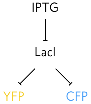
By titrating the amount of IPTG, the expression levels of both YFP and CFP gene products may be controlled. Systematically varying ITPG concentration produced the results shown below:

df_noise_int = pd.read_csv(
    os.path.join(data_path, "elowitz_2002_noise_vs_intensity.csv")
)

df_noise_int["total noise"] = np.sqrt(
    df_noise_int["intrinsic noise"] ** 2 + df_noise_int["extrinsic noise"] ** 2
)

p = bokeh.plotting.figure(
    frame_height=250,
    frame_width=350,
    x_axis_type="log",
    x_axis_label="normalized fluorescent intensity",
    y_axis_label="noise",
)
p.circle(
    source=df_noise_int,
    x="normalized fluorescent intensity",
    y="intrinsic noise",
    legend_label="intrinsic",
)
p.circle(
    source=df_noise_int,
    x="normalized fluorescent intensity",
    y="extrinsic noise",
    legend_label="extrinsic",
    color="orange",
)
p.square(
    source=df_noise_int,
    x="normalized fluorescent intensity",
    y="total noise",
    legend_label="total",
    color="#2ca02c",
)

bokeh.io.show(p)

In the data above, intrinsic noise decays monotonically with increasing expression level, as one would expect from uncorrelated

At high expression level, the copy number of LacI is low. We nonetheless see low intrisic and extrinsic noise because of the high copy numbers of the fluorophore gene product (the denominator in the noise is large). When low fluorescence intensity is observed, the intrinsic and extrinsic noise are both large, as we would expect, since the copy number of gene product is so low. However, when the IPTG concentration is very low (and therefore expression is also low), the resulting the high copy numbers of LacI dampen out extrinsic noise, leading to its drop at low intensity values.

We note that at full induction, the total noise is somewhere around 0.1. By contrast, a “good” electronic circuit has a signal to noise ratio of about 25 or 30 dB, or a noise level of about 0.001, 100 times quieter than this example of gene expression.

Generative Bayesian modeling of noise

In the above analysis, we assumed we knew nothing about underlying probability distribution generating the data. This means we are not modeling the source of the noise, but are rather defining what we mean by intrinsic and extrinsic noise based on moments of the unknown distribution, which we then estimate with plug-in estimates. We now take an alternative approach, where we propose a generative model for the data. The parameters of this model then define what we mean by intrinsic and extrinsic noise. We use Bayes’s theorem to connect the experimental measurements to the noise, given the model.

One of the beauties of generative modeling is that all assumptions are now, by necessity, explicit. We will again make the same assumptions we did when deriving the plug-in estimates, stating them more clearly here.

• The mean fluorescence is equal for the CFP and YFP channels.

• The copy number is linearly related to the measured fluorescence.

• There is no background fluorescence.

• All noise is inherent to the genetic machinery of the bacteria; there is no measurement error.

• The fluorescent intensity of each cell is independent of all other cells and also identically distributed (i.i.d).

• Although under these assumptions the measured fluorescence should take on discrete values (because the camera on the microscope is digital), we nonetheless model the fluorescence values as continuous.

The assumption of no measurement error was not apparent in the nonparametric analysis we did above. We assumed we knew nothing about the distribution that produced the experimental measurements, but we then chose to interpret the plug-in estimates as they relate to genetic noise, ignoring measurement noise.

To build our parametric model, we must first build a probability distribution for the likelihood of the data. This is the probability distribution describing observation of our data set. Because of the i.i.d. assumption, we can consider a single cell, \(i\). Then, our modeling means we specify the joint probability density function \(P(c_i, y_i\mid \theta_i)\) where \(\theta_i\) is a set of parameters that condition the observations.

We will model this distribution as Normal, such that

\begin{align} c_i \sim \mathrm{Norm}(\mu_i, \sigma_i),\\[1em] y_i \sim \mathrm{Norm}(\mu_i, \sigma_i). \end{align}

Here, \(\sigma_i\) explicitly characterizes within cell variability of expression of the gene of interest; it gives the intrinsic noise. If we assume that every cell experiences the same intrinsic noise, then \(\sigma_i = \sigma\;\forall i\), and

\begin{align} c_i \sim \mathrm{Norm}(\mu_i, \sigma),\\[1em] y_i \sim \mathrm{Norm}(\mu_i, \sigma), \end{align}

or

\begin{align} P(c_i, y_i \mid \mu_i, \sigma) = \frac{1}{2\pi\sigma^2}\exp\left[-\frac{(c_i - \mu_i)^2 + (y_i - \mu_i)^2}{2\sigma^2}\right]. \end{align}

The extrinsic noise affects the expression level of all genes; that is it affects variability in \(\mu_i\). We can model the \(\mu_i\)’s as varying from a “global” value \(\mu\) with standard deviation \(\sigma_\mu\) according to a Gaussian distribution,

\begin{align} \mu_i \sim \mathrm{Norm}(\mu, \sigma_\mu), \end{align}

or

\begin{align} P(\mu_i\mid \mu, \sigma_\mu) = \frac{1}{\sqrt{2\pi\sigma_\mu^2}}\,\exp\left[-\frac{(\mu_i-\mu)^2}{2\sigma_\mu^2}\right]. \end{align}

The parameter \(\sigma_\mu\) is related to the extrinsic noise. We can therefore define the intrinsic and extrinsic noise as

\begin{align} &\eta_\mathrm{int} = \frac{\sigma}{\mu},\\[1em] &\eta_\mathrm{ext} = \frac{\sigma_\mu}{\mu}. \end{align}

To complete the generative model, we need to specify prior distributions on the parameters \(\mu\), \(\sigma\), and \(\sigma_\mu\); that is, we need to specify \(P(\mu, \sigma, \sigma_\mu)\). We will leave that unspecified for now, and will proceed to write down Bayes’s theorem for this hierarchical model.

\begin{align} P(\{\mu_i\}, \mu, \sigma, \sigma_\mu\mid \{c_i, y_i\}) \propto \left(\prod_{i=1}^N P(c_i, y_i \mid \mu_i, \sigma) P(\mu_i\mid \mu, \sigma_\mu)\right) P(\mu, \sigma, \sigma_\mu). \end{align}

Performance of full Bayesian inference on this model involves some sophisticated techniques involving Markov chain Monte Carlo, which we will not cover here, but you can explore in an end-of-chapter problem. Most important for this chapter is that we can build a generative model and directly and intuitively interpret its parameters.

References

• Elowitz, et al., Stochastic gene expression in a single cell, Science, 297, 1183–1186, 2002. (link)

Computing environment

%load_ext watermark
%watermark -v -p numpy,pandas,bokeh,jupyterlab

Python implementation: CPython
Python version       : 3.8.13
IPython version      : 8.3.0

numpy     : 1.21.5
pandas    : 1.4.2
bokeh     : 2.4.2
jupyterlab: 3.3.2