10a. Stability diagrams by numerical computation of eigenvalues

[1]:

# Colab setup ------------------
import os, sys, subprocess
if "google.colab" in sys.modules:
    cmd = "pip install --upgrade watermark"
    process = subprocess.Popen(cmd.split(), stdout=subprocess.PIPE, stderr=subprocess.PIPE)
    stdout, stderr = process.communicate()
# ------------------------------

import numpy as np
import scipy.optimize

import bokeh.io
import bokeh.plotting

bokeh.io.output_notebook()

Loading BokehJS ...

In this technical appendix, we demonstrate how to compute a linear stability diagram by “brute force,” in which we grid up parameter space, compute the linear stability matrix, and then numerically compute its eigenvalues and assess them.

Example system: A simple delay circuit

Recall in the Chapter 10 that we consider a circuit with \(N\) intermediates between mRNA and the autorepressive protein product it codes for. Here, we will consider the simplest case with \(N = 1\), shown below.

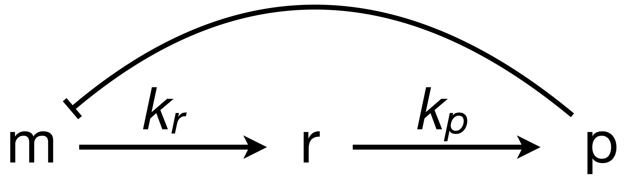
The dimensionless ODEs for this system are

\begin{align} &\frac{\mathrm{d}m}{\mathrm{d}t} = \frac{\beta}{1 + p^n} - m,\\[1em] \kappa^{-1}\,&\frac{\mathrm{d}r}{\mathrm{d}t} = m - r,\\[1em] \gamma^{-1}\,&\frac{\mathrm{d}p}{\mathrm{d}t} = r - p. \end{align}

There is a single fixed point \((m_0, r_0, p_0)\) for this system with \(m_0 = r_0 = p_0\) given by

\begin{align} \beta = m_0(1+m_0^n). \end{align}

We can perform linear stability analysis about this fixed point. The linearized system of ODEs for the perturbations is

\begin{align} \frac{\mathrm{d}}{\mathrm{d}t}\begin{pmatrix} \delta m \\ \delta r \\ \delta p \end{pmatrix} = \mathsf{A}\cdot\begin{pmatrix} \delta m \\ \delta r \\ \delta p \end{pmatrix}, \end{align}

with

\begin{align} \mathsf{A} = \begin{pmatrix} -1 & 0 & -b \\ \kappa & -\kappa & 0 \\ 0 & \gamma & -\gamma \end{pmatrix}, \end{align}

where

\begin{align} b = \frac{\beta n m_0^{n-1}}{(1+m_0^n)^2} = \frac{n m_0^n}{1+m_0^n}. \end{align}

To find the eigenvalues, we write the characteristic polynomial as

\begin{align} -(1+\lambda)(\kappa+\lambda)(\gamma + \lambda) - b \kappa \gamma = -\lambda^3 - (1 + \gamma + \kappa)\lambda^2 - (\gamma + \kappa + \gamma\kappa)\lambda - (1 + b)\gamma \kappa = 0. \end{align}

This polynomial has no positive real roots and either one or three negative real roots according to the Descartes Sign Rule. We are interested in the case where we have one negative real root and two complex conjugate roots. If the real part of these complex conjugate roots is positive, we have an oscillatory instability.

Computing a linear stability diagram by brute force

We can compute the eigenvalues of the linear stability matrix for various values of \(\beta\) and \(\gamma\) for fixed Hill coefficient \(n\). We will take a “brute force” approach and grid up \(\beta\)-\(\gamma\) space and compute the eigenvalues for each set of parameter values and determine if that point is stable or not. We can then display the linear stability diagram as an image, where a pixel is light colored in a stable region and dark colored in an unstable region.

The first step in this brute force calculation is finding the fixed point. We know that the fixed point satisfies \(m_0(1+m_0^n) - \beta = 0\). The fixed point must lie between zero and \(\beta\), so we can use Brent’s method, as discussed in Technical Appendix 9c, to find the root.

[2]:

def fixed_point(beta, n):
    """Computes fixed point for the m⟶r⟶p autorepression system.
    """
    return scipy.optimize.brentq(
        lambda x: x * (1 + x ** n) - beta,
        0,
        beta,
    )

Next, we write a function to compute whether or not the fixed point is linearly stable for a given set of parameters \(\beta\), \(\kappa\), \(\gamma\), and \(n\). The steps are simple:

Compute the fixed point.
Compute the linear stability matrix, which is dependent on the value of the fixed point.
Compute the eigenvalues of the linear stability matrix.
Return True if the real parts of all eigenvalues are negative and False otherwise.

[3]:

def lin_stab(beta, gamma, kappa, n):
    """Returns True if delay system is linearly stable and False
    otherwise.
    """
    # Find fixed point as a function of beta and n
    m_0 = fixed_point(beta, n)

    # Linear stability matrix
    b = n * m_0 ** n / (1 + m_0 ** n)
    A = np.array([[-1, 0, -b], [kappa, -kappa, 0], [0, gamma, -gamma]])

    # Compute eigenvalues
    lam = np.linalg.eigvals(A)

    # Return True is all eigenvalues have negative real parts
    return (lam.real < 0).all()

With this function in hand, we scan values of the parameters for stability. Unfortunately, this is a four-dimensional scan, since we have four dimensionless parameters to consider, \(\beta\), \(\gamma\), \(\kappa\), and \(n\). To limit the parameters we will scan, we can make some physical arguments about \(\kappa\). Recall that \(\kappa = k_r / \gamma_m\), the ratio of the rate constant for production of intermediate from mRNA to the total rate constant for mRNA loss, including loss of mRNA due to possible conversion to the intermediate. If we assume that conversion to intermediate dominates mRNA loss, then \(\gamma_m \approx k_r\) and \(\kappa \approx 1\). Conversely, if the mRNA is not converted to the intermediate, but rather the intermediate is some product derived from, but not consuming, the mRNA, then \(\gamma_m \ne k_r\). We may then have \(\kappa < 1\) if mRNA decay is rapid compared to formation of intermediates, and \(\kappa > 1\) if it is not.

For our first calculation, we will take \(\kappa = 1\) and \(n = 10\) for high ultrasensitivity of repression.

[4]:

def stab_image(kappa, n):
    """Compute "image" of linear stability in the γ-β plane
    for given values of κ and n.
    """
    # beta and gamma values to consider
    beta_vals = np.logspace(0, 4, 200)
    gamma_vals = np.logspace(-2, 2, 200)

    # Compute the linear stability diagram
    stab = np.empty((len(beta_vals), len(gamma_vals)))
    for i, beta in enumerate(beta_vals):
        for j, gamma in enumerate(gamma_vals):
            stab[i, j] = lin_stab(beta, gamma, kappa, n)

    return stab


# Compute stability for kappa = 1 and n = 10
stab = stab_image(1, 10)

To plot the results, we will use the image() method of a Bokeh figure. It expects a list of two-dimensional arrays to render as images. For us, we will include a single image, which we have defined as the 2D array stab in the above cell. The image() method also expects keyword arguments x and y, which specify the coordinates of the bottom left corner of the image as it sits on a set of axes. We also supply dw and dh keyword arguments to specify the width and height, respectively, of the image in the units of the axes in which it resides. These x, y, ,dw, and dh keyword arguments are crucial in this application because we need to properly match up the axis values (the values of \(\beta\) and \(\gamma\)) with the “image” of stability we are plotting. We will also pass a palette keyword argument to specify how the stable and unstable regions are colored and also an alpha keyword argument specifying the opacity of the displayed image.

[5]:

# Plot the result (shaded region has oscillatory instability)
p = bokeh.plotting.figure(
    frame_height=250,
    frame_width=250,
    x_axis_label="γ",
    y_axis_label="β",
    x_axis_type="log",
    y_axis_type="log",
    x_range=[0.01, 100],
    y_range=[1, 10000],
    title="κ = 1, n = 10",
)

# Plot an image with Bokeh; encapsulate 2D array as a liest
p.image([stab], x=0.01, y=1, dw=100, dh=10000, palette="Greys3", alpha=0.5)

# Annotate stable and unstable regions
p.text(x=0.45, y=100, text=["unstable"])
p.text(x=10, y=2, text=["stable"])

bokeh.io.show(p)

We can repeat the calculation for less ultrasensitive repression, this time with \(n = 9\).

[6]:

# Compute stability for kappa = 1 and n = 9
stab = stab_image(1, 9)

# Plot the result
p = bokeh.plotting.figure(
    frame_height=250,
    frame_width=250,
    x_axis_label="γ",
    y_axis_label="β",
    x_axis_type="log",
    y_axis_type="log",
    x_range=[0.01, 100],
    y_range=[1, 10000],
    title="κ = 1, n = 9",
)
p.image([stab], x=0.01, y=1, dw=100, dh=10000, palette="Greys3", alpha=0.5)

bokeh.io.show(p)

The unstable region got thinner as \(n\) decreased. In fact it vanishes for \(n = 8\). Importantly, we see that we must have very high ultrasensitivity to get oscillatory instabilities for reasonable values of \(\beta\) and \(\gamma\). Furthermore, the sliver of parameter space that gives an oscillatory instability is small. For such a simple mechanism for delay, the presence of oscillations are not robust to variations in parameter values and high sensitivity is necessary.

Computing environment

[7]:

%load_ext watermark
%watermark -v -p numpy,scipy,bokeh,jupyterlab

Python implementation: CPython
Python version       : 3.11.3
IPython version      : 8.12.0

numpy     : 1.24.3
scipy     : 1.10.1
bokeh     : 3.2.0
jupyterlab: 3.6.3