13. Promiscuous receptor-ligand interactions increase the bandwidth and specificity of cell-cell communication systems

---

Design principles

• Promiscuous receptor-ligand interactions enable complex responses to combinations of ligands

• These complex response functions enable a given ligand profile to uniquely address more distinct sets of cell types than they could in a fully orthogonal one-ligand one-receptor system.

Techniques

• EQTK can rapidly solve large systems of equilbirium binding reactions.

• Low-dimensional representations of complex system behaviors enable large parameter explorations.

Key Papers

• Y. Antebi et al, “Combinatorial Signal Perception in the BMP Pathway,” Cell, 2017

• C. Su et al, “Ligand-receptor promiscuity enables cellular addressing,” Cell Systems, 2022

• H. Klumpe et al, “The context-dependent, combinatorial logic of BMP signaling,” Cell Systems, 2022

---

# Colab setup ------------------
import os, sys, subprocess
if "google.colab" in sys.modules:
    cmd = "pip install --upgrade eqtk watermark"
    process = subprocess.Popen(cmd.split(), stdout=subprocess.PIPE, stderr=subprocess.PIPE)
    stdout, stderr = process.communicate()
# ------------------------------

import numpy as np
import tqdm

import biocircuits
# import biocircuits.apps
import eqtk

import bokeh.io

import biocircuits.apps
notebook_url = 'localhost:8888'

bokeh.io.output_notebook()

Loading BokehJS ...

Cell-cell communication systems use families of partly redundant ligands and receptors

In a multicellular organism, cells of different types are in constant conversation with one another to ensure correct development and coordinate their many different activities. These conversations are carried out by communication circuits that secrete, sense, and process specific signaling molecules called ligands.

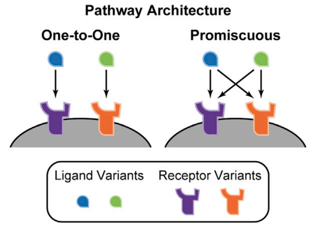
How would you design the ideal cell-cell communication system? You would start with a secreted ligand, to convey the signal, and a corresponding receptor, to sense it. You would probably want your ligand to be extremely specific for your receptor, to avoid undesired crosstalk with other communication pathways. In fact, most core signaling systems are based on pathway-specific ligands and receptors. Once you created your pathway and saw that it was working well, you might want to expand its bandwidth, by adding additional ligands and receptors that function similarly, but independently. That way one ligand could transmit one kind of information through one receptor and a second could independently transmit different information through a distinct receptor. In this way, you could create many “orthogonal” communication channels from a single design. In fact, synthetic biologists have developed precisely this paradigm to create signaling architectures, such as “SynNotch”, that can support multiple independent channels.

You might expect that evolution would have produced a similarly sensible design. However, when we look at many natural communication pathways we see something quite different. As with our hypothetical ideal system, we find not one, but many, homologous ligands per pathway. We also observe many different receptor variants within a pathway. But instead of a one-to-one relationship between a given ligand variant and a corresponding receptor variants, we observe “promiscuous” relationships, in which each ligand interact, to varying extents, with multiple receptors, and each receptor, conversely, interacts with multiple ligands. This occurs in the Wnt, FGF, Notch, Eph-ephrin, and Bone Morphogenetic Protein (BMP) pathways, among many others.

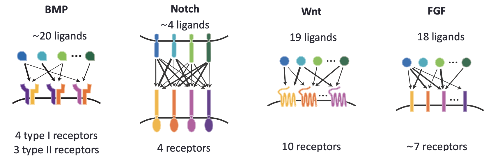
The extraordinary promiscuity in these pathways is perplexing. If all of these different ligand-receptor complexes activate the same downstream targets, then it seems like the cell cannot necessarily “know” which ligand and receptor were involved in a given signaling interaction. That information appears, at least at first glance, to be “lost.”

So, what could account for the prevalence of promiscuous ligand-receptor interactions? Perhaps they do not offer any direct functional advantage, but rather reflect the process through which biological systems evolve through gene duplication and gradual divergence–an evolutionary artifact. Or, perhaps they allow regulatory flexibility, permitting stronger or weaker expression or activity in one tissue relative to another. A third possibility is that, by acting as partly redundant “backups” for one another, these additional ligand and receptors variants increase the robustness of signaling. A final possibility is that these promiscuous interactions provide some other, more direct, signal processing function. While any or all of these may be true, here we focus on this last case – a direct role in signal processing.

Examining different promiscuous ligand-receptor systems a little closer, one notices a few common themes:

• First, the strengths of interactions between different ligands and receptors typically vary quantitatively. Some interactions are strong, and others are weak or even effectively non-existent.

• Second, different ligand and receptor variants are often similar enough to replace each other in some, but not all, contexts. They are partly, but not fully, interchangeable.

• Third, organisms typically do not use a single ligand and a single receptor in most processes. Rather, they appear to use multiple ligands and receptors together in various overlapping combinations.

These observations together suggest that ligands and receptors may be working together in a combinatorial fashion.

The Bone Morphogenetic Protein (BMP) pathways signals through a set of promiscuously interacting ligands and receptors

To gain insight into signal processing by promiscuous ligand-receptor interactions, we will focus on the BMP pathway as an example.

The BMP pathway is part of a larger pathway called TGF-β. The first thing to know about it is that, despite its name, it is not at all specific to bone, but rather functions in virtually all tissue contexts in the body. Its ligands are morphogens that can diffuse away from the site at which they are produced to activate cells at a distance, and for this reason it plays key roles in developmental patterning. Also, because of its eponymous bone-inducing properties, it is used clinically in some orthopedic contexts. Finally, BMP, like most of the core communication pathways, is dysregulated in many diseases.

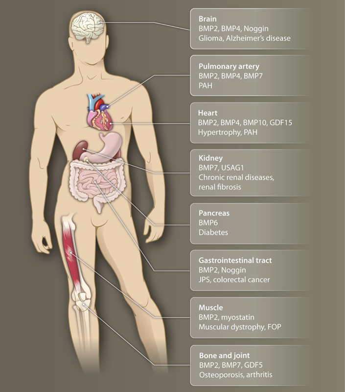
Image taken fromWagner, et al., Sci. Signaling, 2010.

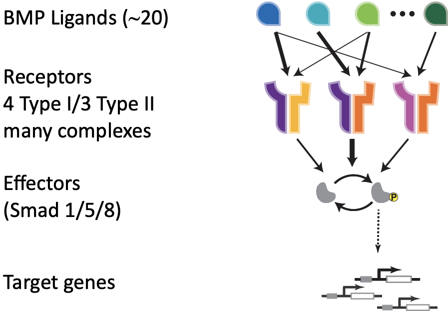
At the molecular level, the BMP pathway includes about 20 different ligands (depending on how you count). A complete BMP receptor is a heterotetramer composed of two type I and two type II subunits. There are 4 different type I and 3 different type II receptor variants that can combine to form a large set of potential heterotetrameric combinations. Different cell types express different combinations of these components, typically including multiple type I or type II subunit variants. The different ligands interact, to varying extents, with each of these receptor complexes to form hundreds or even thousands of different ligand-receptor signaling complexes. These complexes in turn phosphorylate effector proteins Smad1, Smad5, and Smad8, which can then transit to the nucleus to activate target genes.

The mystery here is why this pathway has so much apparent combinatorial complexity. Why not keep it simple and just use a family of ligands and a family of cognate receptors, with no promiscuity, no combinations, and no seemingly unecessary complexity?

If we could answer this question, we might better understand and control the BMP pathway to manipulate a broad range of cellular behaviors.

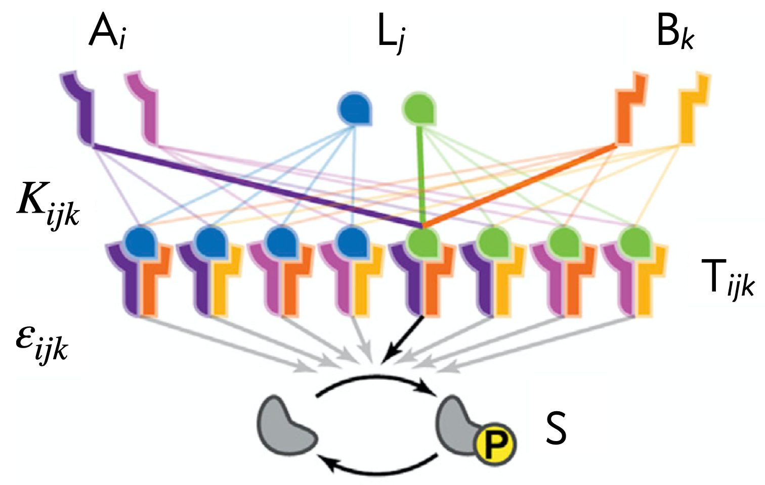
Do BMPs “compute?”

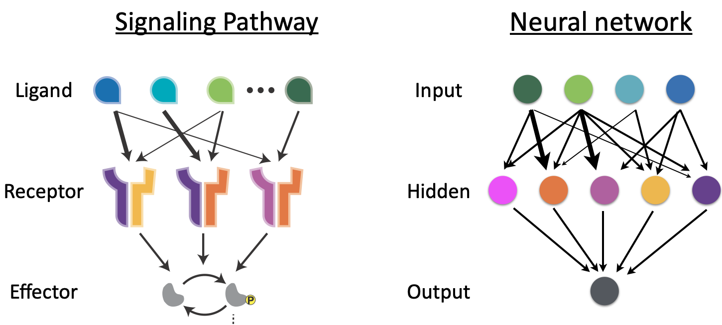
The many-to-many relationship between ligands and receptors may remind you of an artificial neural network. Juxtaposing the diagrams, one can intuit a loose analogy between these two very different types of promiscuous systems. In neural networks, inputs are encoded in a set of input nodes, each of which can activate, with different strengths and in a many-to-many fashion, a second layer of ‘hidden’ nodes. These in turn may activate additional layers of hidden nodes that finally converge to control one or more output nodes. Artificial neural networks are powerful computing architectures that now underlie much of the software we use every day.

Do promiscuous ligand-receptor interactions “compute?” That is, do they calculate complex, combinatorial functions of their ligand inputs?

A clue that the pathway might be computing something interesting comes from analyzing the response of the pathway to combinations of two different ligands. One way to do this is by engineering a reporter cell line that expresses a fluorescent protein reporter in response to pathway activation, and then exposing that reporter cell line to a matrix of different concentrations of two ligands. This was performed by Antebi et al. (2017, Cell), who obtained results that looked like the following.

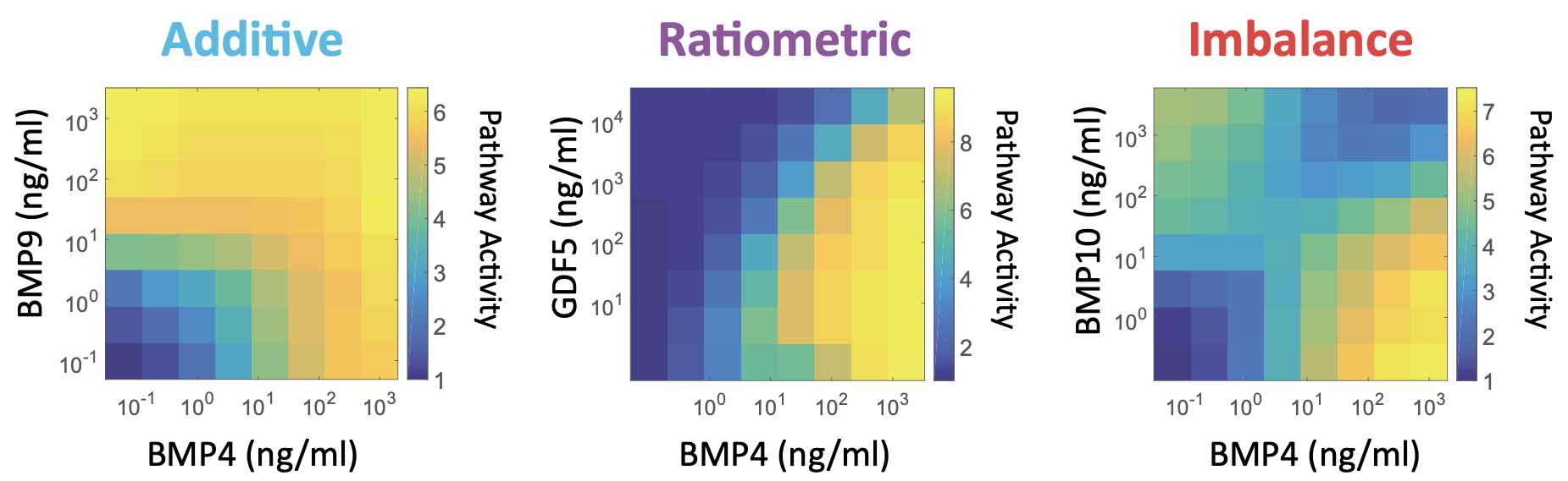
In all of these plots, the x-axis represents the concentration of the same ligand: BMP4. What differs is which second ligand one mixes it with. The example on the left shows that BMP4 and BMP9 combine additively, such that the response of the pathway to the two ligands (heat map color) is about what you would expect given their individual effects.

In the center, we see that GDF5 (another BMP ligand) acts as a dose-dependent inhibitor of activation by BMP4. In this case, the output of the pathway is approximately proportional [BMP4]/[GDF5]. In that sense the pathway “computes” the ratio of these two ligand concentrations.

On the right, we see the most interesting case: BMP4 and BMP10 each activate individually, but when one combines them at the “wrong” proportions, they can neutralize each other’s effects. Because the response is strongest when the ligand concentrations are out of balance, this response can be called an imbalance detector.

Interestingly, these and other functions produced by the pathway often become dependent only on relative levels of different ligands, at least when total ligand concentrations are sufficiently high. Sensing relative ligand levels may be more robust than sensing absolute concentrations by normalizing away variations in the accessibility of a cell to the extracellular medium, absolute receptor concentrations, and other variables that are likely to vary unpredictably. (A similar type of ratiometric sensing has also been observed in yeast, which respond to the ratios of different sugars).

A simple model of promsiscuous ligand-receptor interactions can explain pathway computations

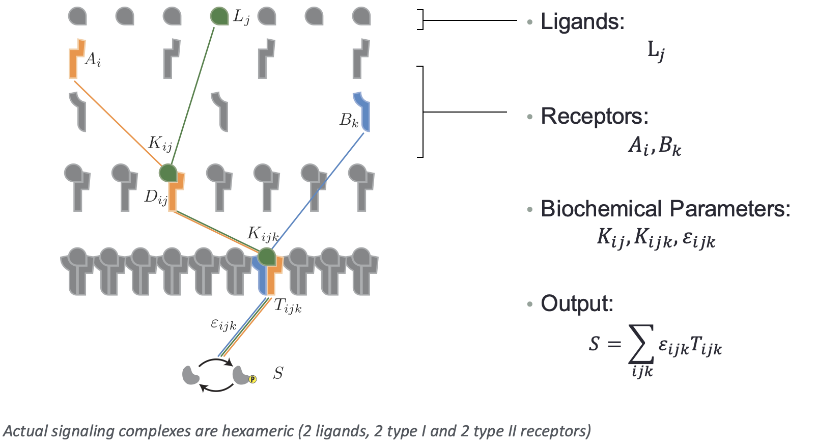
How could these functions arise? To think about that, we will focus on a simplified model of promiscuous ligand-receptor interactions described by Su et al (Cell Systems, 2022). The model considers a family of ligands, denoted \(L_j\), as well as sets of type I and II receptors, denoted \(A_i\) and \(B_k\).

In this model, we will assume that a ligand \(L_j\), a type I receptor \(A_i\), and a type II receptor \(B_k\) independently bind together in a trimolecular reaction to form an active complex \(T_{ijk}\) with an affinity of \(K_{ijk}\). Each trimeric singaling complex \(T_{ijk}\) has its own specific activity (the rate of phosphorylating Smad effector proteins), denoted \(\varepsilon_{ijk}\). The signaling activity is governed by the concentration of phosphorylated Smad, \(s\), given by

\begin{align} s = \sum_{i,j,k} \varepsilon_{ijk}\,t_{ijk}, \end{align}

again using our convention that lowercase symbols denote concentrations. Thus, the activity of the pathway as a whole can be computed by summing up the product of each signaling complex times its individual activity parameter.

This model is a simplification of the natural system, which includes two type I and two type II subunits in each signaling complex, but this simplification will allow us to more easily understand basic principles of combinatorial signaling. Perhaps even more critically, the trimolecular reaction in which three proteins come together simultaneously is explicitly unphysical—in reality, two of the monomers would bind together first to form a dimer, and then the third monomer would bind to this dimer to form the full trimeric complex. These binding events could happen in different sequences. However, for the sake of reducing the complexity of the model and the number of biophysical parameters, we will go ahead and assume this trimolecular form, and later show that relaxing this assumption does not violate the key qualitative conclusions discussed here.

Equations of the one-step promiscuous ligand-receptor model

To compute the signaling activity we need to find the concentrations of all signaling complexes, \(t_{ijk}\). To do so, we assume that the ligand-receptor complexes come to fast equilibrium such that

\begin{align} K_{ijk} = \frac{a_i\,l_j\,b_k}{t_{ijk}}\;\;\forall\;i,j,k. \end{align}

We also enforce conservation of mass, such that the total amount of each kind of receptor is accounted for,

\begin{align} a_i^0 = a_i + \sum_{j,k}t_{ijk} \;\;\forall\;i,\\[1em] b_k^0 = b_i + \sum_{i,j}t_{ijk} \;\;\forall\;k. \end{align}

The ligand concentration is considered differently. To mimic the experimental cell culture environment, where the volume of media is large, and ligand concentrations are not significantly perturbed by the binding of ligands to the relatively small absolute number of receptors expressed by cells, the concentration of a ligand may be considered fixed.

To see what kinds of responses this simplified model can produce, we begin with a minimal instance, containing just two ligand variants, L₁ and L₂, two type A receptors, A₁ and A₂, and two type B receptors, B₁ and B₂. The distribution of ligand-receptor complexes is then controlled by eight equilibrium binding reactions,

\begin{align} \mathrm{A}_i + \mathrm{L}_j + \mathrm{B}_k \rightleftharpoons \mathrm{T}_{ijk}, \end{align}

for all combinations of \((i, j, k) \in [1, 2]\).

The EQTK python package enables solution of coupled equilibria

Solving this model requires evaluating the steady-state values of each complex \(\mathrm{T}_{ijk}\). These are uniquely determined by the values of the binding constants \(K_{ijk}\) and the total concentrations of \(a_i^0\) and \(b_k^0\). However, numerically computing these values is nontrivial.

In this section, we will demonstrate how to use the EQTK (EQuilbirium ToolKit) package to rapidly calculate the steady-state concentrations of the species in coupled equilibria as we have here.

We will now define a function that will encode our desired binding reactions into strings with the appropriate formatting for EQTK’s parsers. EQTK can take a single multi-line string to specify the system’s reactions, where in this case each line is a single binding reaction with the syntax

A_i + L_j + B_k <=> T_i_j_k

to indicate the formation of complex \(T_{ijk}\).

def make_rxns(nA, nB, nL):
    """
    Generate trimolecular binding reactions for a system with
    nA, nB, and nL types of Type A receptors, Type B receptors,
    and ligands, respectively. Returns a single string.
    """
    rxns = ""
    for k in range(nB):
        for j in range(nL):
            for i in range(nA):
                rxns += f"A_{i+1} + L_{j+1} + B_{k+1} <=> T_{i+1}_{j+1}_{k+1}\n"
    return rxns

Using this function for the (2, 2, 2) system gives the following result.

nA = nB = nL = 2

print(make_rxns(nA, nB, nL))

A_1 + L_1 + B_1 <=> T_1_1_1
A_2 + L_1 + B_1 <=> T_2_1_1
A_1 + L_2 + B_1 <=> T_1_2_1
A_2 + L_2 + B_1 <=> T_2_2_1
A_1 + L_1 + B_2 <=> T_1_1_2
A_2 + L_1 + B_2 <=> T_2_1_2
A_1 + L_2 + B_2 <=> T_1_2_2
A_2 + L_2 + B_2 <=> T_2_2_2

It may seem notationally cumbersome to have excessive underscores, but they are necessary if we were to have a system with ten or more types of ligands or receptors because we would have double-digit subscripts.

These reactions are in the appropriate format for EQTK’s reaction parser to generate a stoichiometric matrix \(\mathsf{N}\) from the reactions. The eqtk.parse_rxns() function places the stoichiometric matrix in a data frame with the ordering of the columns given by the order in which the chemical species appear in the string containing the reactions. Because we will be doing thousands and thousands of solves as we explore parameter space, we will be using \(\mathsf{N}\) as a Numpy arrays to save on the computational cost of creating and manipulating data frames in eqtk.solve()’s I/O. So, we should make \(\mathsf{N}\) as a Numpy array where the first columns represent receptors of type A, the next columns represent receptors of type B, the next ligands, and finally trimers. We can code this up in a function to make our stoichiometric matrix.

def make_N(nA, nB, nL):
    rxns = make_rxns(nA, nB, nL)
    N = eqtk.parse_rxns(rxns)

    # Sorted names
    names = sorted(N.columns, key=lambda s: (len(s), s))

    # Sorted columns
    N = N[names]

    # As a Numpy array
    return N.to_numpy(copy=True, dtype=float)

We can now build our stoichiometric matrix.

N = make_N(nA, nB, nL)

# Take a look
print(make_N(2, 2, 2))

[[-1.  0. -1.  0. -1.  0.  1.  0.  0.  0.  0.  0.  0.  0.]
 [ 0. -1. -1.  0. -1.  0.  0.  0.  0.  0.  1.  0.  0.  0.]
 [-1.  0. -1.  0.  0. -1.  0.  0.  1.  0.  0.  0.  0.  0.]
 [ 0. -1. -1.  0.  0. -1.  0.  0.  0.  0.  0.  0.  1.  0.]
 [-1.  0.  0. -1. -1.  0.  0.  1.  0.  0.  0.  0.  0.  0.]
 [ 0. -1.  0. -1. -1.  0.  0.  0.  0.  0.  0.  1.  0.  0.]
 [-1.  0.  0. -1.  0. -1.  0.  0.  0.  1.  0.  0.  0.  0.]
 [ 0. -1.  0. -1.  0. -1.  0.  0.  0.  0.  0.  0.  0.  1.]]

In the above matrix, each of the 8 rows corresponds to the 8 binding reactions, in the order specified by the input string. Each column corresponds to the 14 species involved in our model (\(2+2+2=6\) monomers and \(2^3=8\) possible trimeric complexes). The entries of the matrix are integers that represent the stoichiometric change that the species of that column undergoes due to the reaction of that row.

The equilibrium coefficients

Now that we have defined the binding reactions, we can see how varying the equilibrium constants can affect the resulting signaling. To explore this parameter space efficiently, we use a Dirichlet distribution with all parameters set to one. This is equivalent to choosing a uniform distribution, in dimensionless units such that the sum of all \(K_{ijk}\) is equal to \(1\). This sum-to-one requirement is equivalent to arbitrarily setting units for the dissociation constants.

def make_K(nA, nB, nL):
    Kijk_vals = np.random.dirichlet(np.ones(nA*nB*nL))
    return Kijk_vals

Let’s compute a set of equilibrium constants so we can see how the array looks.

# Seed for reproducibility
seedval = 239486234
np.random.seed(seedval)

K = make_K(nA, nB, nL)

with np.printoptions(formatter={'float': '{: 0.3f}'.format}):
    print(f"K_i_j_k values: {K}")
    print(f"Sum of all K_i_j_k values = {np.sum(K)}")

K_i_j_k values: [ 0.324  0.142  0.129  0.164  0.006  0.085  0.053  0.097]
Sum of all K_i_j_k values = 1.0

Scanning ligand concentrations and receptor expression levels

Ligand concentrations: To see what each function looks like, we will scan pathway activity across a two-dimensional space of ligand concentrations. For this, we can select a set of 15 log-uniformly spaced ligand concentrations from \(10^{-3}\) to \(10^3\) in dimensionless units.

Receptor expression levels: Different cell types naturally express different combinations of receptor subunits. These receptor expression profiles can strongly impact the function that is computed. To scan a range of receptor expression levels, we will choose random receptor expression levels within a log-uniform range of \([10^{-3}, 10^3]\).

The following function constructs a set of initial concentrations satisfying these requirements.

def make_c0_grid(nA, nB, nL, n):
    # Ligand concentrations
    cL0 = np.logspace(-3, 3, n)
    cL0 = np.meshgrid(*tuple([cL0]*nL))

    # Initialize c0
    c0 = np.zeros((n**nL, nA + nB + nL + nA*nB*nL))

    # Add ligand concentrations
    for i in range(nL):
        c0[:, i+nA+nB] = cL0[i].flatten()

    # Random concentrations of receptors
    for i in range(nA):
        c0[:, i] = 10**np.random.uniform(-3, 3)
    for i in range(nB):
        c0[:, i + nA] = 10**np.random.uniform(-3, 3)

    return c0

Let’s generate a c0 array and take a look at its shape.

n = 15

c0 = make_c0_grid(nA, nB, nL, n)

c0.shape

(225, 14)

There are 225 different sets of initial concentrations we solve for.

The readout

The concentrations of the respective species are “read out” by the intensity of the intracellular signaling triggered by the ligand-receptor binding. As we have already defined, the signal strength \(s\) is given by

\begin{align} s = \sum_{ijk} \varepsilon_{ijk}\,t_{ijk}. \end{align}

We can write a function to compute this from the parameters \(\varepsilon_{ijk}\) and concentrations returned by eqtk.solve().

def readout(epsilon, c):
    return np.dot(epsilon, c[:, -len(epsilon):].transpose())

The choice of \(\varepsilon_{ijk}\) is drawn out of a uniform distribution subject to the contraint that \(\sum_{ijk} \varepsilon_{ijk} = 1\). We can again accomplish this by drawing out of a Dirichlet distribution.

def make_epsilon(nA, nB, nL):
    return np.random.dirichlet(np.ones(nA * nB * nL))

# Set seed for reproducibility
np.random.seed(seedval)
epsilon = make_epsilon(nA, nB, nL)

Solve!

To solve for set of coupled equilibria, we could use the eqtk.solve() function. In that case, it allows all concentrations to vary as it finds the set of concentrations of all species that satisfy equilibrium. In this case, as we mentioned before, we are setting the ligand concentration to be fixed. EQTK enables fixing some concentrations, in which case the eqtk.fixed_value_solve() function is used. This function also takes an array fixed_c the specifies the fixed concentrations, if any, of any species. This array is the same shape as the c0 array, and contains negative numbers or NaNs if a given concentration is not fixed.

Since the ligand concentrations are fixed, and they are in columns 4 and 5 of c0, we need to build fixed_c with those columns containing the constant ligand concentrations.

fixed_c = -np.ones_like(c0)
fixed_c[:, 4:6] = c0[:, 4:6]

We now have all the ingredients to solve for the concentrations and compute the readout.

c = eqtk.fixed_value_solve(c0=c0, fixed_c=fixed_c, N=N, K=K)
s = readout(epsilon, c)

We can make a heat map of the readout as a function of ligand concentration, bearing in mind that the initial ligand concentrations are in columns 4 and 5 of c0.

def heatmap(c0, s, n):
    """Make a heatmap of responses."""

    # Generate x, y, and z arrays for plot
    x = c0[:n, 4]
    y = c0[::n, 5]
    z = s.reshape((n, n))

    # Clean the plot a bit by overriding the tick labels
    xtick_overrides = ["" for x_ in x]
    xtick_overrides[0] = "0.001"
    xtick_overrides[len(xtick_overrides) // 2] = "1"
    xtick_overrides[-1] = "1000"
    ytick_overrides = xtick_overrides

    # Build heat map
    p = biocircuits.viz.heatmap(
        x,
        y,
        z,
        xtick_overrides=xtick_overrides,
        ytick_overrides=ytick_overrides,
        log_color=True,
        colorbar=False,
        x_axis_label="L₁",
        y_axis_label="L₂",
    )

    return p

bokeh.io.show(heatmap(c0, s, n))

And we are done! The heatmap you see above shows the value of the pathway activation strength,

\begin{align} s = \sum_{ijk} \varepsilon_{ijk}\,t_{ijk}, \end{align}

as a function of different concentrations of ligands \(\mathrm{L}_1\) and \(\mathrm{L}_2\) for a single instantiation in parameter space (\(\mathrm{K}_{ijk}\) and \(\varepsilon_{ijk}\) are fixed), where each point in the heatmap has a random concentration profile of the Type A and Type B receptors.

At first glance this response function looks a bit like an OR gate on its input ligands, with \(s\) increasing alongside increasing concentrations of either of its input ligands. But we notice that \(\mathrm{L}_1\)’s maximal activation of the pathway is weaker than that of \(\mathrm{L}_2\), and furthermore we see that there is a slight antisynergistic effect where increasing \(\mathrm{L}_1\) can slightly decrease \(s\) when the \(\mathrm{L}_2\) concentration is high.

We can see, then, that this type of promiscuous binding interaction can create nontrivial response functions even in a simple system that only contains 2 types of each component. But is this the only type of behavior that can occur with this system architecture? If we chose different values for the \(\mathrm{K}_{ijk}\) and \(\varepsilon_{ijk}\), would we see a different response profile?

We would like to search over many different parameter values to try and answer this question, but it would be impractical to print out a heatmap like the one above for every single choice of our thousands of points in parameter space that we would like to sample and look at it by eye to see if we find any interesting behaviors. We must therefore come up with a low-dimensional representation of the response function shown in the heatmap in order to make the results of our parameter search interpretable.

Rapid characterization of signaling behavior

In order to obtain a summary measure that captures the relevant information about the response function, Antebi et al. considered only the portions of the response associated with high ligand concentrations (the top row and rightmost column of the heatmap above, marked by a white border). They then defined the following quantities:

variable	description
\(a\)	Signaling level of weaker ligand in absence of stronger ligand
\(b\)	Signaling level of stronger ligand in absence of weaker ligand
\(c\)	Maximum signal in the high-ligand concentration region of the heat map
\(d\)	Minimum signal in the high-ligand concentration region of the heat map

In the heat map above, \(\mathrm{L}_1\) is the weaker ligand because at high ligand concentration, it has a lower activation of the pathway (\(S\)).

From these parameters, they defined two summary measures: the relative ligand strength, \(\mathrm{RLS} = a/b\), which ranges from zero to one, and the ligand interference coefficient, \(\mathrm{LIC} = d/a - b/c\).

We will now randomly select equilibrium constants, receptor concentrations, and readout magnitudes \(\varepsilon_{ijk}\) and compute the RLS and LIC. We can then make a plot of LIC vs. RLS to explore the range of response behaviors this system can exhibit.

Because we only need to compute equilibria in the high ligand concentration regimes to calculate the LIC and RLS, we will write another function that only generates c0 at high ligand concentrations in order to save time by removing unnecessary calculations.

def make_c0_high_ligand(nA, nB, nL, n):
    if nL != 2:
        raise ValueError("Only defined for the two-ligand problem.")

    # Initialize c0
    c0 = np.zeros((2 * n + 1, nA + nB + nL + nA * nB * nL))

    # Ligand concentrations
    cL10 = np.concatenate([[0], np.logspace(-3, 3, n), [1e3] * n])
    cL20 = np.concatenate([[1e3] * n, np.logspace(3, -3, n), [0]])
    c0[:, nA + nB] = cL10
    c0[:, nA + nB + 1] = cL20

    # Random concentrations of receptors
    for i in range(nA):
        c0[:, i] = 10 ** np.random.uniform(-3, 3)
    for i in range(nB):
        c0[:, i + nA] = 10 ** np.random.uniform(-3, 3)

    # Concentration of fixed ligands
    fixed_c = -np.ones_like(c0)
    fixed_c[1:-1, 4:6] = c0[1:-1, 4:6]

    return c0, fixed_c

Let’s look at how the ligand concentrations are represented in c0.

c0_high, fixed_c_high = make_c0_high_ligand(nA, nB, nL, n)

c0_high[:, 4:6]

array([[0.00000000e+00, 1.00000000e+03],
       [1.00000000e-03, 1.00000000e+03],
       [2.68269580e-03, 1.00000000e+03],
       [7.19685673e-03, 1.00000000e+03],
       [1.93069773e-02, 1.00000000e+03],
       [5.17947468e-02, 1.00000000e+03],
       [1.38949549e-01, 1.00000000e+03],
       [3.72759372e-01, 1.00000000e+03],
       [1.00000000e+00, 1.00000000e+03],
       [2.68269580e+00, 1.00000000e+03],
       [7.19685673e+00, 1.00000000e+03],
       [1.93069773e+01, 1.00000000e+03],
       [5.17947468e+01, 1.00000000e+03],
       [1.38949549e+02, 1.00000000e+03],
       [3.72759372e+02, 1.00000000e+03],
       [1.00000000e+03, 1.00000000e+03],
       [1.00000000e+03, 3.72759372e+02],
       [1.00000000e+03, 1.38949549e+02],
       [1.00000000e+03, 5.17947468e+01],
       [1.00000000e+03, 1.93069773e+01],
       [1.00000000e+03, 7.19685673e+00],
       [1.00000000e+03, 2.68269580e+00],
       [1.00000000e+03, 1.00000000e+00],
       [1.00000000e+03, 3.72759372e-01],
       [1.00000000e+03, 1.38949549e-01],
       [1.00000000e+03, 5.17947468e-02],
       [1.00000000e+03, 1.93069773e-02],
       [1.00000000e+03, 7.19685673e-03],
       [1.00000000e+03, 2.68269580e-03],
       [1.00000000e+03, 1.00000000e-03],
       [1.00000000e+03, 0.00000000e+00]])

The concentration of L1 varies from 0 to 1000 while L2 is held fixed at 1000. Then, L2 varies from 1000 to 0 while L1 is held fixed at 1000.

Finally, we need a function to compute the LIC and RLS. Knowing the structure of the c0_high arrays helps in this task.

def lic_rls(s, n):
    a = s[0]
    b = s[-1]
    c = np.max(s)
    d = np.min(s)

    # Ensure a is the low level.
    if a > b:
        a, b = b, a

    lic = d / a - b / c
    rls = a / b

    return lic, rls

We are now ready to solve for the LIC and RLS for many random parameter sets. Running the cell below will take a couple of minutes.

n_sets = 10000

rls = np.empty(n_sets)
lic = np.empty(n_sets)

# List to store parameters
parameters = [None for _ in range(n_sets)]

# Create list of seed values for reproducibility
np.random.seed(1234)
seed_vals = np.random.randint(low=1, high=999999999, size=(2, n_sets))

for i in tqdm.tqdm(range(n_sets)):
    c0_high, fixed_c_high = make_c0_high_ligand(nA, nB, nL, n)

    # Set seed for Ks
    np.random.seed(seed_vals[0,i])
    K = make_K(nA, nB, nL)

    # Set seed for epsilons
    np.random.seed(seed_vals[1,i])
    epsilon = make_epsilon(nA, nB, nL)
    parameters[i] = dict(receptor_conc=c0_high[0,:4], K=K, epsilon=epsilon)

    c = eqtk.fixed_value_solve(c0=c0_high, fixed_c=fixed_c_high, N=N, K=K)
    s = readout(epsilon, c)
    lic[i], rls[i] = lic_rls(s, n)

100%|████████████████████████████████████████████████████████████████████████| 10000/10000 [02:15<00:00, 73.94it/s]

Let’s plot the results!

p = bokeh.plotting.figure(
    frame_height=200,
    frame_width=400,
    x_range=[-1, 1],
    y_range=[0, 1],
    x_axis_label="ligand interference coefficient",
    y_axis_label="relative ligand strength",
    tools=["pan,box_zoom,wheel_zoom,hover,save,reset"],
    tooltips=[("index", "@index")]
)

source = bokeh.models.ColumnDataSource(dict(lic=lic, rls=rls, index=np.arange(n_sets)))

p.circle(source=source, x="lic", y="rls", size=3, fill_alpha=0, line_alpha=0.3, line_color="black")

bokeh.io.show(p)

We see that most of the points have a LIC value of 0, but that there is some low-density spread of LIC values in both the positive and negative directions. Perhaps these points might exhibit some interesting response behavior?

Since we stored the parameters in a list of dictionaries, we can easily hover over a specific point on the RLS vs. LIC plot to view its index, and then make a full heatmap with those parameters.

For example, index 7234 (one of the upper-left points) might be interesting.

i = 7234

K = parameters[i]["K"]
c0 = make_c0_grid(nA, nB, nL, n)
c0[:,:4] = parameters[i]["receptor_conc"]
epsilon = parameters[i]["epsilon"]

c = eqtk.fixed_value_solve(c0=c0, fixed_c=fixed_c, N=N, K=K)
s = readout(epsilon, c)

bokeh.io.show(heatmap(c0, s, n))

This is an “imbalance” condition, where high signaling occurs when either \(\mathrm{L}_1\) or \(\mathrm{L}_2\) have high concentration, but not when they the concentrations are similar to each other. It therefore acts similar to an XOR gate, but instead of acting purely on the concentrations of the inputs, it also acts on the ratio of these concentrations.

What about another point? Let’s consider index 5312, which is one of the points with a LIC and RLS are both close to 0.

i = 5312

K = parameters[i]["K"]
c0 = make_c0_grid(nA, nB, nL, n)
c0[:,:4] = parameters[i]["receptor_conc"]
epsilon = parameters[i]["epsilon"]

c = eqtk.fixed_value_solve(c0=c0, fixed_c=fixed_c, N=N, K=K)
s = readout(epsilon, c)

bokeh.io.show(heatmap(c0, s, n))

This point in parameter space gives a ratiometric repsonse, where the pathway activates when the ratio \(l_1 / l_2\) is high. Let’s look at one more point, this time index 8936 on the upper right.

i = 8936

K = parameters[i]["K"]
c0 = make_c0_grid(nA, nB, nL, n)
c0[:,:4] = parameters[i]["receptor_conc"]
epsilon = parameters[i]["epsilon"]

c = eqtk.fixed_value_solve(c0=c0, fixed_c=fixed_c, N=N, K=K)
s = readout(epsilon, c)

bokeh.io.show(heatmap(c0, s, n))

This is a response function that was not observed experimentally! We will call it a ‘Balance’ function because the pathway is maximally activated when the concentrations of \(\mathrm{L}_1\) and \(\mathrm{L}_2\) are equal to each other, in addition to being above a minimal threshold.

Determining the causes of the response functions

We have now seen that the model is able to generate a variety of different response functions, but one question we have not yet answered is why the model sometimes generates one response function and sometimes generates another. Thankfully, because we saved all the parameter values associated with each point in (RLS, LIC) space, we can choose a particular point with a known response function and back out the actual \(K_{ijk}\) and \(\varepsilon_{ijk}\) values that define that point. Looking at common trends in the relationships between the parameter values that yield a given response function, we can then start to get insights into the potential mechanistic sources of these response functions.

Performing such an analysis, Su et al. concluded that the response functions arise due to particular relationships between the \(K_{ijk}\) values and the \(\varepsilon_{ijk}\) values. The schematic on the bottom row of the figure below represents the system with 2 ligand types and 2 of each receptor type, like we have examined. The top set of arrows represent the \(K_{ijk}\) values and the bottom set of arrows represent the \(\varepsilon_{ijk}\) values, with thicker arrows representing a stronger value (tight binding via low \(K_{ijk}\) or strong activation via high \(\varepsilon_{ijk}\)). Blue arrows represent the parameters associated with the \(\mathrm{L}_1\) ligand while green arrows represent the parameters associated with the \(\mathrm{L}_2\) ligand.

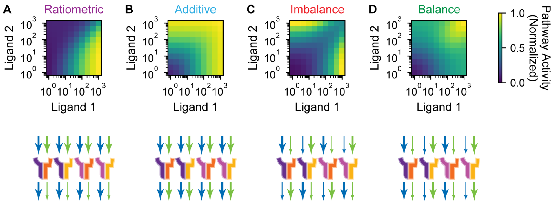
Think through each of these schematics— does it make sense to you that they would lead to the given response? For example, in the Ratiometric response, both ligands bind to both receptor types with equal affinity, but complexes that contain ligand 1 activate the downstream pathway strongly, while complexes that contain ligand 2 activate the downstream pathway weakly. This means that if the concentraiton of ligand 2 is higher than that of ligand 1, then most of the receptors will be bound up in weakly-activating complexes, making the total pathway activation low. On the other hand, if the concentration of ligand 1 is higher than that of ligand 2, then most of the receptors will instead be bound up in complex of the strongly-activating form, making the total pathway activation high. It is therefore through these sequestration effects that emerge from the promiscuous interactions that these complex response functions are able to emerge.

Removing the trimolecular binding assumption from the model

At this point, we have now seen that our simple model for the BMP system can capture a variety of different response functions to two ligand inputs, and in particular can reproduce the three experimentally-observed response functions. But is this result a quirk of the specific assumptions we made in setting up our model? In particular, we might be concerned about the presence of trimolecular binding events— perhaps the model’s reliance on such unphsyical reactions are causing it to generate unrealistic outputs.

We will therefore modify our model to relax this trimolecular binding assumption. This new model follows the structure that was used in Antebi et al.

The major change between this model and the previous one-step binding model is that we now explicitly require the trimer to form by two successive bimolecular binding reactions, where a ligand \(L_j\) first binds a Type A receptor \(A_i\) to form a dimer \(D_{ij}\), which then binds to a Type B receptor \(B_k\) to form a trimer \(T_{ijk}\). Our equations for the model are therefore

\begin{align} &\mathrm{D}_{ij} \rightleftharpoons \mathrm{A}_i + \mathrm{L}_j \\[1em] &\mathrm{T}_{ijk} \rightleftharpoons \mathrm{D}_{ij} + \mathrm{B}_k, \\[1em] &s = \sum_{ijk} \varepsilon_{ijk}\,t_{ijk}. \end{align}

A dashboard for the two-step binding model

As above, we can use EQTK to solve the two-step model. We have developed a dashboard below that you can use to explore the model by changing the values of of the various \(K_{ij}\) (binding constants for the dimer-formation reactions) and the \(K_{ijk}\) (binding constants for the trimer-forming reactions) values.

As you can see by the four preset parameter values included in the dashboard, the model can still produce the four types of response functions that we observed in the one-step model. Can you find any other types of response functions?

bokeh.io.show(
   biocircuits.apps.promiscuous_222_app(), notebook_url=notebook_url
)

Ligand-receptor promiscuity enables cellular addressing

Now that we have seen these complex response functions that are possible through the promiscuous interactions of the BMP sysytem, however, we might ask what functional consequence these response functions might have beyond their direct application of enabling the cells to compute and respond to ratios of different input signals. In particular, a natural question would be whether such a promiscuous architecture would allow a given ligand profile to selectively activate, or address, a larger number of cell types than a corresponding nonpromiscuous one-to-one architecture with the same diversity of ligand and receptor types.

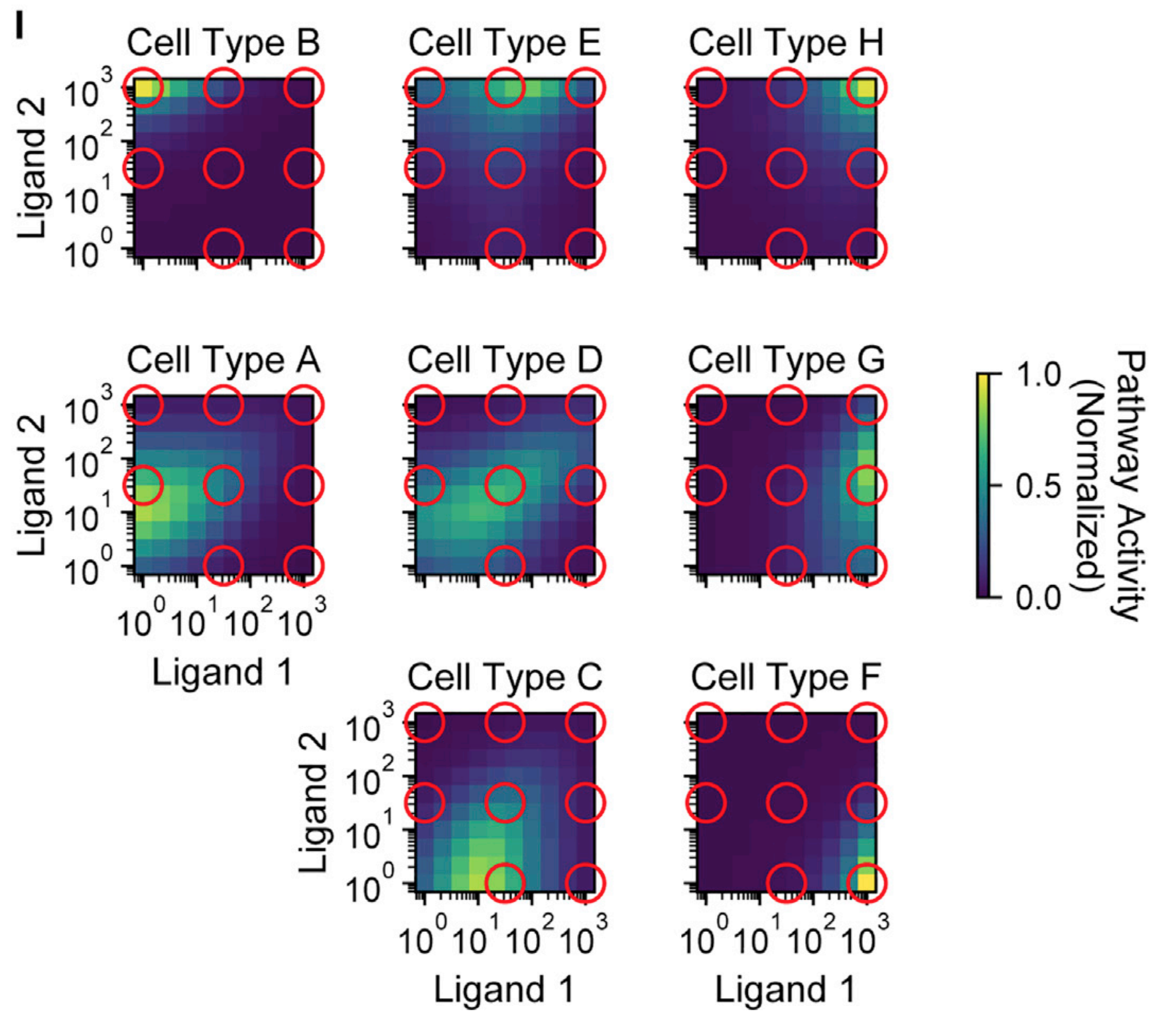
Su et al. investigated this question, and found that a promiscuous architecture can indeed increase the bandwidth of cellular addressing. As the diversity of receptor types is increased, the model can generate even more distinct response behaviors than those we explored above. For example, in the heatmaps below, we see that a system with 4 type A receptors and 3 type B receptors can, even when only two ligand types are present, uniquely address eight different cell types that are distinguished by different expression profiles of the various receptors, simply by expressing different concentration profiles of these two ligands.

Looking forward: what is the ‘grammar’ of BMP signaling?

We have now seen that by understanding this combinatorial logic of BMP signaling, we may be able to understand how the cell uses this pathway to target specific cell types to help orchestrate developmental processes. An immediate implication of this understanding is that we might be able to leverage this knowledge to manually target these cell types for therapeutic purposes. However, all of our analyses so far have relied on smaller, more interpretable case studies that only involve two ligand types. How can we scale up our understanding of the BMP pathway to the complexity we see in nature, where there are ten major distinct BMP ligands?

As we saw earlier in our parameter screen, this is another situation where low-dimensional representations are required in order to navigate a high-dimensional space. While previously this space was the space of the many different parameters, here this space expands further to include the many possible ligand and receptor types as well. What sort of low-dimensional representation would be useful here to navigate such a huge combinatorial space?

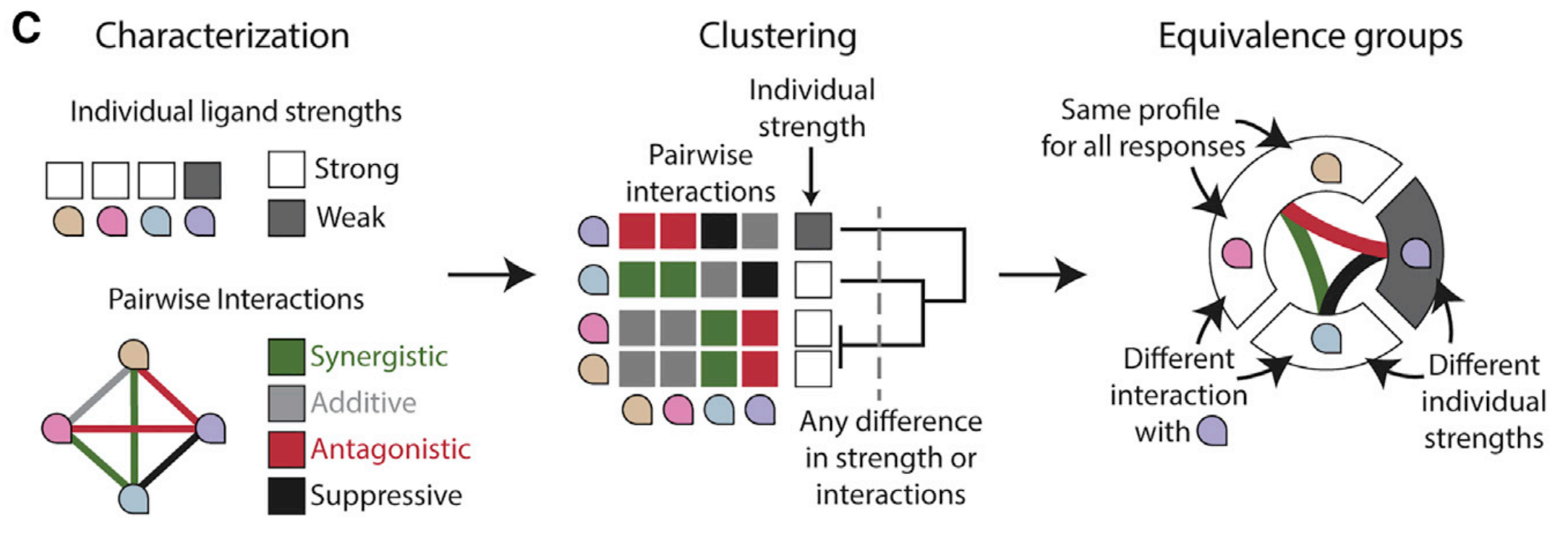
Klumpe et al. (2022, Cell Systems) had the insight to, instead of coming up with different measures and trying to force them onto the data, to instead directly ask the cells themselves what sort of low-dimensional representation they themselves might be using. The authors took various cell types, distinguished by their receptor expression profiles, and screened them against all pairwise combinations of all 10 BMP ligands, and noted whether the two ligands in a pair acted synergistically or antisynergistically with each other for a given cell type. Importantly, this screen then allowed the authors to determine whether any set of ligands had the same interactions with a given partner ligand. Any set of ligands where all the ligands had the same interaction profile with all other ligands would be, from the point of view of this cell type, functionally identical to each other. The authors termed this an ‘equivalence class’, as schematized below.

While such a strict requirement for equivalence might seem like it would rarely ever occur, the authors found that all seven cell types that they tested showed strong equivalence behavior between many of the BMP ligands, as shown in the figure below. In fact, some of the equivalence classes were quite large, with some cell types treating eight distinct BMP ligands as funtionally equivalent!

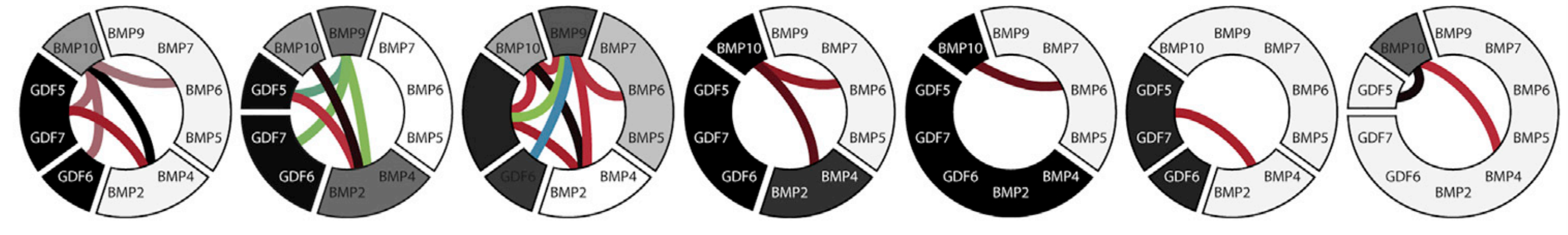
These data suggest that one potential consequence of a promiscuous interaction system with many different ligand/receptor types is that any given cell type will interpret several of these components as functionally equivalent, and that such redundancy may be a required part of the increased addressing bandwidth enabled by such architectures.

Through their work, Klumpe et al. were therefore able to accomplish the first step in determining what sort of representation the cells themselves are using when presented with a particular set of BMP ligands— we now know that, whatever the representation is, it must interpret these particular sets of ligand types as equivalent. This knowledge allows us to place a constraint on the possible representations that could exist, and by placing additional constraints on these possible representations, we will eventually be able to hone in on the true ‘grammar’ by which cells compute and respond to BMP signals. This is the frontier of the field, and so we ask you: what would be the next constraint you would try to place, and how would you set up an experiment to do so?

Computing environment

%load_ext watermark
%watermark -v -p numpy,tqdm,eqtk,biocircuits,bokeh,jupyterlab

Python implementation: CPython
Python version       : 3.10.10
IPython version      : 8.12.0

numpy      : 1.23.5
tqdm       : 4.65.0
eqtk       : 0.1.3
biocircuits: 0.1.12
bokeh      : 3.1.0
jupyterlab : 3.5.3

---

Problems

• 13.1: Programming cellular response