3a. Nondimensionalization
Recall our differential equation for the dynamics of an autoactivator,
\begin{align} \frac{\mathrm{d}x}{\mathrm{d}t} = \beta\, \frac{(x/k)^n} {1 + (x/k)^n} - \gamma x. \end{align}
Here we can identify two variables, \(x\) and \(t\), and four parameters, \(\beta\), \(\gamma\), \(k\), and \(n\). Understanding how the circuit behaves as four parameters are varied is challenging. However, the dynamics do not depend on all four parameters independently. In a simpler case, we saw that for unregulated expression, the steady state protein concentration is given by the ratio \(\beta/\gamma\). It is the ratio that matters, not the individual values of \(\beta\) and \(\gamma\). We will start this foray into nondimensionalization using this example.
Why nondimensionalize?
The procedure of nondimensionalization allows us to reduce the number of independent parameters and still be able to explore the full dynamics. The key idea is that each variable or parameter has some dimension. For example, \(x\) has dimension of concentration, or number of particles per cubic length, written as
\begin{align} x = \left[\frac{N}{L^3}\right]. \end{align}
Similarly, the parameter \(\gamma\) has dimension of inverse time, or \(\gamma = [T^{-1}]\). It is clear that each term in the dynamical equation has dimension of \(N/L^3 T\). In general, every term in an equation must have the same dimension; trying to add, for example, a meter to a kilogram is nonsensical.
The nondimensionalization procedure involves rewriting the equations such that every term is dimensionless, which means that every term has dimension of unity. This is beneficial for several reasons.
It reduces the number of parameters you need to consider. Only dimensionless ratios/products of parameters are considered.
It allows comparison of the relative magnitudes of terms in an equation.
It provides intuition by identifying which ratios and products of parameters control the dynamics.
The Buckingham π Theorem
The Buckingham π Theorem allows us to know how many dimensionless variables and parameters we will have for a given problem. The theorem states:
A system described by \(n\) variables and parameters, built from \(r\) independent dimensions, is completely described by \(p = n - r\) dimensionless groups.
Let us apply the theorem to the autoactivation system. We start by listing all of the parameters and their dimension.
parameter/variable |
dimension |
|---|---|
\(x\) |
\(N/L^3\) |
\(t\) |
\(T\) |
\(\beta\) |
\(N/L^3T\) |
\(k\) |
\(N/L^3\) |
\(\gamma\) |
\(T^{-1}\) |
\(n\) |
dimensionless |
We have \(n = 6\) variables and parameters and \(r = 2\) independent dimensions. We might be tempted to think that \(r = 3\), but note that \(N\) and \(L\) always appear as the ratio \(N/L^3\), which is a concentration. Therefore \(N\) and \(L\) are not independent. Our two independent dimensions are then \(T\) and \(N/L^3\). We therefore can cast this problem in terms of four dimensionless groups. We are free to choose them how we like, but as we will see below, it is convenient to choose them to be \(\gamma t\), \(x/k\), \(\beta/k\gamma\) and \(n\).
Procedure for nondimensionalization
Although the Buckingham π Theorem tells us many dimensionless groups will be present, there is no single algorithmic procedure to determine those groups for a given set of dynamical equations. In the context of systems biology, we have found the following procedure to be generally effective.
Let \(\theta\) be one of the variables in a dynamical equation, including space and time. In the above dynamical equations, \(\theta\) could be either \(x\) or \(t\). (There are no spatial variables in this problem. Also, recall that \(\beta\), \(\gamma\), \(k\), and \(n\) are system parameters, not variables.)
For each variable (including time), define a dimensionless version (which we will usually mark with a tilde) such that \(\theta = \theta_d \tilde{\theta}\), where \(\theta\) is some variable. Here, \(\tilde{\theta}\) is called a dimensionless variable, and the constant \(\theta_d\) imparts the dimension of \(\theta\) (hence the subscript d).
Substitute these expressions into the dynamical equations.
Rearrange the equations such that every term is dimensionless. As a result, you find ratios and products of the \(\theta_d\)’s and the system parameters. These ratios are dimensionless and are called dimensionless parameters.
Choose expressions for the \(\theta_d\)’s that minimize the number of dimensionless parameters. The number of dimensionless variables plus the number of dimensionless parameters will be \(p\) given by the Buckingham π Theorem.
As usual, this is best seen by example. In the case of the simple autoactivator circuit, the two \(\theta\)’s are \(x\) and \(t\). We start be defining
\begin{align} &t = t_d\,\tilde{t},\\[1em] &x = x_d\,\tilde{x}. \end{align}
Substituting these into the dynamical equation, we obtain
\begin{align} \frac{x_d}{t_d}\frac{\mathrm{d}\tilde{x}}{\mathrm{d}\tilde{t}} = \beta\,\frac{(x_d\tilde{x}/k)^{n}}{1 + (x_d\tilde{x}/k)^{n}} - \gamma x_d\tilde{x}. \end{align}
We now want to make every term dimensionless. To do that, we divide both sides of the equation by \(x_d/t_d\) to give
\begin{align} \frac{\mathrm{d}\tilde{x}}{\mathrm{d}\tilde{t}} = \frac{\beta\,t_d}{x_d}\,\frac{(x_d\tilde{x}/k)^{n}}{1 + (x_d\tilde{x}/k)^{n}} - \gamma\,t_d\, \tilde{x}. \end{align}
Looking at the above expression, we can immediately see that if we set \(x_d = k\) then the terms inside the activating Hill term will become dimensionless, yielding
\begin{align} \frac{\mathrm{d}\tilde{x}}{\mathrm{d}\tilde{t}} = \frac{\beta\,t_d}{k}\,\frac{\tilde{x}^{n}}{1 + \tilde{x}^{n}} - \gamma\,t_d\, \tilde{x}. \end{align}
At this point, we have two dimensionless variables, \(\tilde{x} = x/k\) and \(\tilde{t} = t/t_d\), and three dimensionless parameters, \(\beta\,t_d/k\), \(\gamma\,t_d\), and \(n\). The Buckingham π Theorem tells us that we will end up with four, so we can still eliminate one of the dimensionless parameters. We can do this by choosing \(t_d = \gamma^{-1}\), which yields
\begin{align} \frac{\mathrm{d}\tilde{x}}{\mathrm{d}\tilde{t}} = \frac{\beta}{\gamma\,k}\,\frac{\tilde{x}^{n}}{1 + \tilde{x}^{n}} - \tilde{x}. \end{align}
We now have two dimensionless parameters and two dimensionless variables. We define the dimensionless production rate as
\begin{align} \tilde{\beta} = \frac{\beta}{\gamma\,k}, \end{align}
giving our dimensionless dynamical equation
\begin{align} \frac{\mathrm{d}\tilde{x}}{\mathrm{d}\tilde{t}} = \tilde{\beta}\,\frac{\tilde{x}^{n}}{1 + \tilde{x}^{n}} - \tilde{x}. \end{align}
We now see that the entire nondimensional dynamics of our system can be described using only two parameters, \(\tilde{\beta}\) and \(n\).
As an added bonus, nondimensionalization makes clear what dimensionless parameters, which are ratios of dimensional parameters, are important for the dynamics. It is always important to reason about what the dimensionless parameters represent. In this case, we already know that \(n\) is the Hill coefficient, which represents the ultrasensitivity of the gene’s regulation. We see from its definition that \(\tilde{\beta} = \beta/\gamma k\) is the ratio of the gene’s unregulated steady state (which we know from Chapter 1 to be \(\beta/\gamma\)) and the Hill activation parameter \(k\), the concentration of X at which the activation of its regulated gene is half-maximal. In other words, \(\tilde{\beta}\) can be interpreted as a ratio of X’s unregulated steady state expression level to the level of X necessary to activate itself.
Because tildes can be notionally cumbersome, we will often drop them for convenience, writing redefinition of parameters and variables as, for this example,
\begin{align} &t \leftarrow \gamma t,\\[1em] &x \leftarrow x/k,\\[1em] &\beta \leftarrow \beta/\gamma k, \end{align}
such that
\begin{align} \frac{\mathrm{d}x}{\mathrm{d}t} = \beta\,\frac{x^{n}}{1 + x^n} - x. \end{align}
Nondimensionalization of the Collins toggle switch system
As another example of a nondimensionalization procedure, let use consider the two-repressor positive feedback loop of the engineered toggle switch.
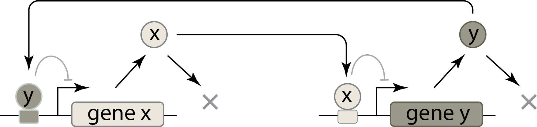
The dynamical equations for the X and Y proteins, assuming for simplicity that they share the same Hill coefficient \(n\) and neglecting the dynamics associated with using the inducer signals to inactivate a particular repressor, are
\begin{align} &\frac{dx}{dt} = \frac{\beta_x}{1 + (y/k_y)^n} - \gamma_x x,\\[1em] &\frac{dy}{dt} = \frac{\beta_y}{1 + (x/k_x)^n} - \gamma_y y. \end{align}
The variables and parameters and their dimensions are
parameter/variable |
dimension |
|---|---|
\(x\) |
\(N_x/L^3\) |
\(y\) |
\(N_y/L^3\) |
\(t\) |
\(T\) |
\(\beta_x\) |
\(N_x/L^3T\) |
\(\beta_y\) |
\(N_y/L^3T\) |
\(k_x\) |
\(N_x/L^3\) |
\(k_y\) |
\(N_y/L^3\) |
\(\gamma_x\) |
\(T^{-1}\) |
\(\gamma_y\) |
\(T^{-1}\) |
\(n\) |
dimensionless |
We have \(n = 10\) variables and parameters and \(r = 3\) independent dimensions, \(N_x/L^3\), \(N_y/L^3\), and \(T\). The Buckingham π Theorem says we should be able to express these dynamics in terms of seven dimensionless groups. We have three variables, so that leave four dimensionless parameters.
We make our usual definitions, \(x = x_d\,\tilde{x}\), \(y = y_d\,\tilde{y}\), and \(t = t_d\,\tilde{t}\). Substituting these into the dynamical equations gives
\begin{align} &\frac{x_d}{t_d}\,\frac{d\tilde{x}}{d\tilde{t}} = \frac{\beta_x}{1 + (y_d\,\tilde{y}/k_y)^n} - \gamma_x\,y_d\, \tilde{x},\\[1em] &\frac{y_d}{t_d}\,\frac{d\tilde{y}}{d\tilde{t}} = \frac{\beta_y}{1 + (x_d\,\tilde{x}/k_x)^n} - \gamma_y\,y_d\, \tilde{y}. \end{align}
Dividing the respective equations by \(x_d/t_d\) and \(y_d/t_d\) to make every term dimensionless gives
\begin{align} &\frac{d\tilde{x}}{d\tilde{t}} = \frac{\beta_x\,t_d}{x_d}\,\frac{1}{1 + (y_d\,\tilde{y}/k_y)^n} - \gamma_x\,t_d\, \tilde{x},\\[1em] &\frac{d\tilde{y}}{d\tilde{t}} = \frac{\beta_y\,t_d}{y_d}\,\frac{1}{1 + (x_d\,\tilde{x}/k_x)^n} - \gamma_y\,t_d\, \tilde{y}. \end{align}
Choosing \(x_d = k_x\) and \(y_d = k_y\) cleans up the Hill functions, giving
\begin{align} &\frac{d\tilde{x}}{d\tilde{t}} = \frac{\beta_x\,t_d}{k_x}\,\frac{1}{1 + \tilde{y}^n} - \gamma_x\,t_d\, \tilde{x},\\[1em] &\frac{d\tilde{y}}{d\tilde{t}} = \frac{\beta_y\,t_d}{k_y}\,\frac{1}{1 + \tilde{x}^n} - \gamma_y\,t_d\, \tilde{y}. \end{align}
We currently have eight dimensionless groups, so we can eliminate one (and only one) more by choosing the timescale \(t_d\). There are several choices we could make. We could choose \(t_d = k_x/\beta_x\), \(t_d = k_y / \beta_y\), \(t_d = \gamma_x^{-1}\), or \(t_d = \gamma_y^{-1}\). These respectively are the time scales of producing enough X to get repression, of producing enough Y to get repression, of decay of X, and of decay of Y. We will choose the decay time of X as our timescale, setting \(t_d = \gamma_X^{-1}\). With this choice, we have
\begin{align} &\frac{d\tilde{x}}{d\tilde{t}} = \frac{\beta_x}{\gamma_x\,k_x}\,\frac{1}{1 + \tilde{y}^n} - \gamma_x\,t_d\, \tilde{x},\\[1em] &\frac{d\tilde{y}}{d\tilde{t}} = \frac{\beta_y}{\gamma_x\,k_y}\,\frac{1}{1 + \tilde{x}^n} - \frac{\gamma_y}{\gamma_x}\, \tilde{y}. \end{align}
Because it makes sense to define dimensionless production rates in terms of the decay rate and Hill activation coefficient of the _same_species, we will divide the second equation by \(\gamma_y/\gamma_x\) to give
\begin{align} \frac{\gamma_x}{\gamma_y}\,\frac{d\tilde{y}}{d\tilde{t}} = \frac{\beta_y}{\gamma_y\,k_y}\,\frac{1}{1 + \tilde{x}^n} - \tilde{y}. \end{align}
We can now define dimensionless parameters \(\tilde{\beta}_x = \beta_x / \gamma_x\,k_x\), \(\tilde{\beta}_y = \beta_y / \gamma_y\,k_y\), and \(\gamma = \gamma_y/\gamma_x\), to give
\begin{align} &\frac{d\tilde{x}}{d\tilde{t}} = \tilde{\beta}_x\,\frac{1}{1 + \tilde{y}^n} - \tilde{x},\\[1em] \gamma^{-1}\,&\frac{d\tilde{y}}{d\tilde{t}} = \tilde{\beta}_y\,\frac{1}{1 + \tilde{x}^n} - \tilde{y}. \end{align}
Nondimensionalization of the activator-substrate depletion reaction-diffusion system
To give one more example of nondimensionalization, we will nondimensionalize the activator-substrate depletion system used in the study of reaction-diffusion systems. We will explore this system in Chapter 21. You can read the chapter about the system if you like, but for now we are using its dynamical equations as an instructive example of nondimensionalization when there is a spatial variable. Briefly, this is a reaction-diffusion system where there are two diffusing species, one called an activator with concentration \(a\), and one called a substrate with concentration \(s\). Chemically, the activator catalyzes its own production by consuming substrate. It may also autodegrade. The substrate is constitutively produced and experiences negligible autodegradation. Both species may diffuse with diffusion coefficients \(D_a\) and \(D_s\), respectively. It is useful to know that diffusion coefficients have dimension of \(L^2/T\). The dynamical equations for this model are
\begin{align} &\frac{\partial a}{\partial t} = D_a\,\frac{\partial^2 a}{\partial x^2} + \mu_a\,a^2s - \gamma\,a,\\[1em] &\frac{\partial s}{\partial t} = D_s\,\frac{\partial^2 s}{\partial x^2} + \beta - \mu_s\,a^2s. \end{align}
Note that \(x\) is a spatial variable; it denotes a position along the \(x\)-direction in space and has dimension of length. We can write a table of the variables and parameters with their dimensions.
parameter/variable |
\(\mathbf{\text{dimension}}\) |
|---|---|
\(a\) |
\(N_a/L^3\) |
\(s\) |
\(N_s/L^3\) |
\(x\) |
\(L\) |
\(t\) |
\(T\) |
\(\mu_a\) |
\((N_a N_s L^6 T)^{-1}\) |
\(\mu_s\) |
\((N_a N_s L^6 T)^{-1}\) |
\(\gamma\) |
\(T^{-1}\) |
\(\beta\) |
\(N_s/L^3 T\) |
\(D_a\) |
\(L^2/T\) |
\(D_s\) |
\(L^2/T\) |
We have four independent dimensions, \(L\), \(T\), \(N_a\), and \(N_s\), and ten parameters and variables, which means we can write the system using six dimensionless groups according to the Buckingham π Theorem.
Defining \(a = a_d\,\tilde{a}\), \(s = s_s\,\tilde{s}\), \(t = t_d\,\tilde{t}\), and \(x = x_d\,\tilde{x}\), and substituting into the dynamical equations, we get
\begin{align} &\frac{a_d}{t_d}\,\frac{\partial \tilde{a}}{\partial \tilde{t}} = \frac{D_a\,a_d}{x_d^2}\,\frac{\partial^2 \tilde{a}}{\partial \tilde{x}^2} + \mu_a\,a_d^2\,s_d\,\tilde{a}^2\tilde{s} - \gamma\,a_d\,\tilde{a},\\[1em] &\frac{s_d}{t_d}\,\frac{\partial \tilde{s}}{\partial \tilde{t}} = \frac{D_s\,s_d}{x_d^2}\,\frac{\partial^2 \tilde{s}}{\partial \tilde{x}^2} + \beta - \mu_s\,a_d^2\,s_d\,\tilde{a}^2\tilde{s}. \end{align}
Dividing the respective equations by \(a_d/t_d\) and \(s_d/t_d\) yields
\begin{align} &\frac{\partial \tilde{a}}{\partial \tilde{t}} = \frac{D_a\,t_d}{x_d^2}\,\frac{\partial^2 \tilde{a}}{\partial \tilde{x}^2} + \mu_a\,a_d\,s_d\,t_d\,\tilde{a}^2\tilde{s} - \gamma\,t_d\,\tilde{a},\\[1em] &\frac{\partial \tilde{s}}{\partial \tilde{t}} = \frac{D_s\,t_d}{x_d^2}\,\frac{\partial^2 \tilde{s}}{\partial \tilde{x}^2} + \frac{\beta\,t_d}{s_d} - \mu_s\,a_d^2\,t_d\,\tilde{a}^2\tilde{s}. \end{align}
We are now left with choosing values of \(a_d\), \(s_d\), \(x_d\) and \(t_d\) that will minimize the number of dimensionless parameters. We have four dimensionless variables (\(\tilde{a}\), \(\tilde{s}\), \(\tilde{x}\) and \(\tilde{t}\)), so we should end up with only two dimensionless parameters. To start, we can set the timescale to be \(t_d = \gamma^{-1}\). This amounts to choosing the time scale to be that of autodegratation of the activator. We could choose the length scale to be \(x_d = \sqrt{D_a t_d} = \sqrt{D_a/\gamma}\), corresponding to the distance an activator molecules travels by diffusion before degrading. The eliminates two of the dimensionless parameters. Instead, though, we will choose \(x_d = \sqrt{D_s/\gamma}\), which is the distance a substrate can diffuse before an activator degrades. We are free to make this choice, even though it seems like an odd one, and we do it mostly for historical reasons (see, e.g., Koch and Meinhardt, 1994). The result is
\begin{align} &\frac{\partial \tilde{a}}{\partial \tilde{t}} = \frac{D_a}{D_s}\,\frac{\partial^2 \tilde{a}}{\partial \tilde{x}^2} + \frac{\mu_a\,a_d\,s_d}{\gamma}\,\tilde{a}^2\tilde{s} - \tilde{a},\\[1em] &\frac{\partial \tilde{s}}{\partial \tilde{t}} = \frac{\partial^2 \tilde{s}}{\partial \tilde{x}^2} + \frac{\beta}{\gamma\,s_d} - \frac{\mu_s\,a_d^2}{\gamma}\,\tilde{a}^2\tilde{s}. \end{align}
It is clear that the dimensionless parameter \(D_s/D_a\) will remain, and we still need to eliminate two by choosing \(a_d\) and \(s_d\). We can start by stipulating that
\begin{align} \frac{\mu_a\,a_d\,s_d}{\gamma} = 1 \label{eq:first_nondim} \end{align}
to eliminate the dimensionless parameter in the equation describing the dynamics of the activator. We can stipulate further that the remaining two dimensionless parameters are equal,
\begin{align} \frac{\beta}{\gamma\,s_d} = \frac{\mu_s\,a_d^2}{\gamma}. \label{eq:second_nondim} \end{align}
Thus, we have two equations for the two unknowns, \(a_d\) and \(s_d\). The first equation \eqref{eq:first_nondim} gives
\begin{align} a_d\,s_d = \frac{\gamma}{\mu_a}. \end{align}
and the second equation \eqref{eq:second_nondim} gives
\begin{align} a_d = \frac{\beta}{\mu_s\,a_d\,s_d} = \frac{\beta\mu_a}{\gamma\mu_s}. \end{align}
As a result,
\begin{align} s_d = \frac{\gamma^2\mu_s}{\beta\,\mu_a^2}. \end{align}
Defining
\begin{align} \mu = \frac{\beta}{\gamma\,s_d} = \frac{\mu_s\,a_d^2}{\gamma} = \frac{\beta^2\mu_a^2}{\gamma^3\mu_s} \end{align}
and
\begin{align} d = \frac{D_a}{D_s}, \end{align}
we have identified our two dimensionless parameter and the dimensionless equations are
\begin{align} &\frac{\partial \tilde{a}}{\partial \tilde{t}} = d\,\frac{\partial^2 \tilde{a}}{\partial \tilde{x}^2} + \tilde{a}^2\tilde{s} - \tilde{a},\\[1em] &\frac{\partial \tilde{s}}{\partial \tilde{t}} = \frac{\partial^2 \tilde{s}}{\partial \tilde{x}^2} + \mu(1 - \tilde{a}^2\tilde{s}). \end{align}
The interpretation of the parameter \(d\) is straightforward; it is the ratio of the diffusion coefficients of the activator and substrate. The parameter \(\mu\) looks more convoluted, but inspecting the dimensionless equations reveals that it parametrizes the rate of reactions for production and consumption of substrate compared to those for the production and degration of activator.
References
Koch, A. J. and Meinhardt, H., Biological pattern formation: From basic mechanisms to complex structures, Rev. Mod. Phys., 66, 1481–1507, 1994. (link)
Computing environment
[1]:
%load_ext watermark
%watermark -v -p jupyterlab
Python implementation: CPython
Python version       : 3.10.10
IPython version      : 8.10.0

jupyterlab: 3.5.3