12. Molecular titration generates ultrasensitive responses in biological circuits
Design principle
Molecular titration provides a simple, versatile mechanism to generate ultrasensitive responses in molecular circuits
Molecular titration generates threshold-linear responses to miRNAs.
Molecular titration enables stochastic activation of bacterial persistence states
[1]:
# Colab setup ------------------
import os, sys, subprocess
if "google.colab" in sys.modules:
    cmd = "pip install --upgrade biocircuits watermark"
    process = subprocess.Popen(cmd.split(), stdout=subprocess.PIPE, stderr=subprocess.PIPE)
    stdout, stderr = process.communicate()
# ------------------------------

import numpy as np

import biocircuits

import bokeh.io
import bokeh.plotting

bokeh.io.output_notebook()
Introduction: Molecular titration as an ultrasensitivity module
Biological circuits rely heavily on “switches,” systems in which a change in the level or state of an input molecule can strongly alter the level or state of the output molecules it controls. When we say a process is “switch-like”, we usually mean that a small change in the input can generate a much larger and more complete change in output. In other words, switches are ultrasensitive. (In some contexts, we go further to demand that switches have a toggle-like, or hysteretic, behavior based on bistability.)
Biological circuits are replete with such ultrasensitive switches: The cell cycle uses switches to click decisively from one phase to another. Signal transduction systems require ultrasensitivity to amplify small but important input signals into large responses. Multistable cell fate control systems use switches to enforce distinct cellular states. Natural and synthetic oscillators such as the circadian clock and the repressilator, as we have seen, also require ultrasensitive switches.
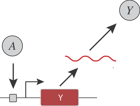
Are there simple, generalizable, engineerable circuit-level design strategies that could confer ultrasensitivity? For instance, consider a simple gene regulatory system, in which an input activator, \(A\), controls the expression of a target protein \(Y\):
Let’s pause to ask:
How could you ensure ultrasensitivity in the transcription response function (dependence of Y on A)?
How could you make the threshold and sensitivity of the response function tunable?
Defining sensitivity and ultrasensitivity
Thus far, we have used the term ultrasensitivity a bit loosely, roughly taking ultrasensitivity to mean a “switch-like” response, quantified by having a Hill coefficient greater than one. Here is a precise definition: An ultrasensitive response is one in which a given fold change in the concentration or activity of an input molecule produces a larger fold change in the level or activity of an output molecule. Because a fold change in a quantity means an incremental change in its logarithm (e.g., \(x \to a x\) means that \(x\) changes by a factor of \(a\), and correspondingly \(\ln x \to \ln a x = \ln a + \ln x\) means that \(\ln x\) changes by an additive amount \(\ln a\)), we define the sensitivity \(s\) of the input-output relationship as
\begin{align} s = \left|\frac{\mathrm{d} \ln y}{\mathrm{d} \ln x}\right| = \frac{x}{y}\left|\frac{\mathrm{d}y}{\mathrm{d} x} \right|, \end{align}
where \(x\) and \(y\) are the concentrations of the respective molecules. If a regulatory interaction is ultrasensitive, then \(s > 1\) for at least some values of \(x\). When discussing ultrasensitivity, we need make clear what operating point we are considering—for example, the “EC50” or point at which the function is half maximal, or, alternatively, the point at which the sensitivity itself is maximized.
Sensitivity of Hill functions
The Hill function provides a versatile way to parameterize ultrasensitive responses.
\begin{align} &y = \frac{(x/k)^{n}}{1 + (x/k)^{n}} \text{ for X activating Y},\\[1em] &y = \frac{1}{1 + (x/k)^{n}} \text{ for X repressing Y}. \end{align}
As a reminder, below are Hill functions for several values of the Hill coefficient, \(n\). Here, in contrast to our original introduction to Hill function in Chapter 1, in the plots on a logarithmic scale, we also have the y-axis in a logarithmic scale so we can more directly visualize the sensitivity
\begin{align} s = \left|\frac{\mathrm{d} \ln y}{\mathrm{d} \ln x}\right|. \end{align}
[2]:
# Values of Hill coefficient
n_vals = [1, 2, 5, 10]

# Compute activator response
x = np.concatenate((np.linspace(0, 1, 200), np.linspace(1, 4, 200)))
x_log = np.concatenate((np.logspace(-2, 0, 200), np.logspace(0, 2, 200)))

f_a = []
f_a_log = []
f_r = []
f_r_log = []
for n in n_vals:
    if n == np.inf:
        f_a.append(np.concatenate((np.zeros(200), np.ones(200))))
        f_a_log.append(f_a[-1])
    else:
        f_a.append(x ** n / (1 + x ** n))
        f_r.append(1 / (1 + x ** n))
        f_a_log.append(x_log ** n / (1 + x_log ** n))
        f_r_log.append(1 / (1 + x_log ** n))

# Build plots
p_act = bokeh.plotting.figure(
    frame_height=225,
    frame_width=350,
    x_axis_label="x/k",
    y_axis_label="activating Hill function",
    x_range=[x[0], x[-1]],
)
p_rep = bokeh.plotting.figure(
    frame_height=225,
    frame_width=350,
    x_axis_label="x/k",
    y_axis_label="repressing Hill function",
    x_range=[x[0], x[-1]],
)

p_act_log = bokeh.plotting.figure(
    frame_height=225,
    frame_width=350,
    x_axis_label="x/k",
    y_axis_label="activating Hill function",
    x_range=[x_log[0], x_log[-1]],
    x_axis_type="log",
    y_axis_type="log",
)
p_rep_log = bokeh.plotting.figure(
    frame_height=225,
    frame_width=350,
    x_axis_label="x/k",
    y_axis_label="repressing Hill function",
    x_range=[x_log[0], x_log[-1]],
    y_range=[1e-21, 1e1],
    x_axis_type="log",
    y_axis_type="log",
)

# Set up toggling between activating and repressing and log/linear
p_act.visible = False
p_rep.visible = False
p_act_log.visible = True
p_rep_log.visible = False

radio_button_group_ar = bokeh.models.RadioButtonGroup(
    labels=["activating", "repressing"], active=0, width=150
)
radio_button_group_log = bokeh.models.RadioButtonGroup(
    labels=["linear", "log"], active=1, width=100
)

col = bokeh.layouts.column(
    p_act,
    p_rep,
    p_act_log,
    p_rep_log,
    bokeh.models.Spacer(height=10),
    bokeh.layouts.row(
        bokeh.models.Spacer(width=55),
        radio_button_group_ar,
        bokeh.models.Spacer(width=75),
        radio_button_group_log,
    ),
)
radio_button_group_ar.js_on_click(
    bokeh.models.CustomJS(
        args=dict(
            radio_button_group_log=radio_button_group_log,
            p_act=p_act,
            p_rep=p_rep,
            p_act_log=p_act_log,
            p_rep_log=p_rep_log,
        ),
        code="""
if (radio_button_group_log.active == 0) {
    if (p_act.visible == true) {
        p_act.visible = false;
        p_rep.visible = true;
    }
    else {
        p_act.visible = true;
        p_rep.visible = false;
    }
}
else {
    if (p_act_log.visible == true) {
        p_act_log.visible = false;
        p_rep_log.visible = true;
    }
    else {
        p_act_log.visible = true;
        p_rep_log.visible = false;
    }
}
""",
    )
)

radio_button_group_log.js_on_click(
    bokeh.models.CustomJS(
        args=dict(
            radio_button_group_ar=radio_button_group_ar,
            p_act=p_act,
            p_rep=p_rep,
            p_act_log=p_act_log,
            p_rep_log=p_rep_log,
        ),
        code="""
if (radio_button_group_ar.active == 0) {
    if (p_act_log.visible == true) {
        p_act_log.visible = false;
        p_act.visible = true;
    }
    else {
        p_act_log.visible = true;
        p_act.visible = false;
    }
}
else {
    if (p_rep_log.visible == true) {
        p_rep_log.visible = false;
        p_rep.visible = true;
    }
    else {
        p_rep_log.visible = true;
        p_rep.visible = false;
    }
}
""",
    )
)

# Color scheme for plots
colors_act = bokeh.palettes.Blues256[32:-32][:: -192 // (len(n_vals) + 1)]
colors_rep = bokeh.palettes.Reds256[32:-32][:: -192 // (len(n_vals) + 1)]

# Populate glyphs
for i, n in enumerate(n_vals):
    legend_label = "n → ∞" if n == np.inf else f"n = {n}"
    p_act.line(x, f_a[i], line_width=2, color=colors_act[i], legend_label=legend_label)
    p_rep.line(x, f_r[i], line_width=2, color=colors_rep[i], legend_label=legend_label)
    p_act_log.line(
        x_log, f_a_log[i], line_width=2, color=colors_act[i], legend_label=legend_label
    )
    p_rep_log.line(
        x_log, f_r_log[i], line_width=2, color=colors_rep[i], legend_label=legend_label
    )

# Reposition legends
p_act.legend.location = "bottom_right"
p_act_log.legend.location = "bottom_right"
p_rep_log.legend.location = "bottom_left"

bokeh.io.show(col)
For an activating Hill function, the sensitivity is
\begin{align} s = \left|\frac{\mathrm{d} \ln y}{\mathrm{d} \ln x}\right| = \frac{n}{1+(x/k)^n}, \end{align}
which is greater than one when \(n > 1\) and \(x/k < (n-1)^{1/n}\). Thus, as a rule of thumb, for regulation described by an activating Hill function, ultrasensitivity is achieved when \(n > 1\) and \(x \ll k\). For \(n \ge 2\), ultrasensitivity is achieved for \(x < k\). By contrast, for \(x > k\), the response is not ultrasensitive, eventually it becoming flat.
Similarly, for a repressive Hill function,
\begin{align} s = \frac{n(x/k)^n}{1+(x/k)^n}, \end{align}
which is greater than one when \(n > 1\) and \(x/k > (n-1)^{1/n}\). Repressive Hill regulation has a similar rule of thumb: for \(n \ge 2\), ultrasensitivity is achieved for \(x > k\).
The plots of sensitivity below demonstrate these rules of thumb.
[3]:
# Values of Hill coefficient
n_vals = [1, 2, 5, 10]

# Compute activator response
x = np.concatenate((np.linspace(0, 1, 200), np.linspace(1, 4, 200)))
x_log = np.concatenate((np.logspace(-2, 0, 200), np.logspace(0, 2, 200)))

s_a = []
s_a_log = []
s_r = []
s_r_log = []
for n in n_vals:
    s_a.append(n / (1 + x ** n))
    s_a_log.append(n / (1 + x_log ** n))
    s_r.append(n * x ** n / (1 + x ** n))
    s_r_log.append(n * x_log ** n / (1 + x_log ** n))

# Build plots
p_act = bokeh.plotting.figure(
    frame_height=225,
    frame_width=350,
    x_axis_label="x/k",
    y_axis_label="sensitivity",
    x_range=[x[0], x[-1]],
)
p_rep = bokeh.plotting.figure(
    frame_height=225,
    frame_width=350,
    x_axis_label="x/k",
    y_axis_label="sensitivity",
    x_range=[x[0], x[-1]],
)

p_act_log = bokeh.plotting.figure(
    frame_height=225,
    frame_width=350,
    x_axis_label="x/k",
    y_axis_label="sensitivity",
    x_range=[x_log[0], x_log[-1]],
    x_axis_type="log",
)
p_rep_log = bokeh.plotting.figure(
    frame_height=225,
    frame_width=350,
    x_axis_label="x/k",
    y_axis_label="sensitivity",
    x_range=[x_log[0], x_log[-1]],
    x_axis_type="log",
)

# Set up toggling between activating and repressing and log/linear
p_act.visible = True
p_rep.visible = False
p_act_log.visible = False
p_rep_log.visible = False

radio_button_group_ar = bokeh.models.RadioButtonGroup(
    labels=["activating", "repressing"], active=0, width=150
)
radio_button_group_log = bokeh.models.RadioButtonGroup(
    labels=["linear", "log"], active=0, width=100
)

col = bokeh.layouts.column(
    p_act,
    p_rep,
    p_act_log,
    p_rep_log,
    bokeh.models.Spacer(height=10),
    bokeh.layouts.row(
        bokeh.models.Spacer(width=55),
        radio_button_group_ar,
        bokeh.models.Spacer(width=75),
        radio_button_group_log,
    ),
)
radio_button_group_ar.js_on_click(
    bokeh.models.CustomJS(
        args=dict(
            radio_button_group_log=radio_button_group_log,
            p_act=p_act,
            p_rep=p_rep,
            p_act_log=p_act_log,
            p_rep_log=p_rep_log,
        ),
        code="""
if (radio_button_group_log.active == 0) {
    if (p_act.visible == true) {
        p_act.visible = false;
        p_rep.visible = true;
    }
    else {
        p_act.visible = true;
        p_rep.visible = false;
    }
}
else {
    if (p_act_log.visible == true) {
        p_act_log.visible = false;
        p_rep_log.visible = true;
    }
    else {
        p_act_log.visible = true;
        p_rep_log.visible = false;
    }
}
""",
    )
)

radio_button_group_log.js_on_click(
    bokeh.models.CustomJS(
        args=dict(
            radio_button_group_ar=radio_button_group_ar,
            p_act=p_act,
            p_rep=p_rep,
            p_act_log=p_act_log,
            p_rep_log=p_rep_log,
        ),
        code="""
if (radio_button_group_ar.active == 0) {
    if (p_act_log.visible == true) {
        p_act_log.visible = false;
        p_act.visible = true;
    }
    else {
        p_act_log.visible = true;
        p_act.visible = false;
    }
}
else {
    if (p_rep_log.visible == true) {
        p_rep_log.visible = false;
        p_rep.visible = true;
    }
    else {
        p_rep_log.visible = true;
        p_rep.visible = false;
    }
}
""",
    )
)

# Color scheme for plots
colors_act = bokeh.palettes.Blues256[32:-32][:: -192 // (len(n_vals) + 1)]
colors_rep = bokeh.palettes.Reds256[32:-32][:: -192 // (len(n_vals) + 1)]

# Populate glyphs
for i, n in enumerate(n_vals):
    legend_label = f"n = {n}"
    p_act.line(x, s_a[i], line_width=2, color=colors_act[i], legend_label=legend_label)
    p_rep.line(x, s_r[i], line_width=2, color=colors_rep[i], legend_label=legend_label)
    p_act_log.line(
        x_log, s_a_log[i], line_width=2, color=colors_act[i], legend_label=legend_label
    )
    p_rep_log.line(
        x_log, s_r_log[i], line_width=2, color=colors_rep[i], legend_label=legend_label
    )

# Reposition legends
p_rep.legend.location = "top_left"
p_rep_log.legend.location = "top_left"

bokeh.io.show(col)
Ultrasensitivity ≠ gain
Note that ultrasensitivity is different than gain. A system in which \(y = 100 x\) has high gain, but still responds linearly to its input, and is therefore not ultrasensitive.
[4]:
p = bokeh.plotting.figure(
    frame_width=200,
    frame_height=200,
    x_axis_label="input x",
    y_axis_label="output y",
    tools=["save"],
    x_range=[0, 1],
    y_range=[0, 2],
    title='𝑁𝑜𝑡 ultrasensitive!'
)

p.xaxis.ticker = []
p.yaxis.ticker = []

p.line([0, 1], [0, 0.5], line_width=2)
p.line([0, 1], [0, 1], line_width=2)
p.line([0, 1], [0, 2], line_width=2)
p.line([0, 1], [0, 4], line_width=2)
p.text(
    x=[0.75], y=[0.4], text=["low gain"], angle=np.arctan(0.25), text_font_size="8pt"
)
p.text(
    x=[0.65],
    y=[0.675],
    text=["medium gain"],
    angle=np.arctan(0.5),
    text_font_size="8pt",
)
p.text(
    x=[0.65], y=[1.325], text=["high gain"], angle=np.arctan(1), text_font_size="8pt"
)
p.text(
    x=[0.31], y=[1.3], text=["very high gain"], angle=np.arctan(2), text_font_size="8pt"
)

bokeh.io.show(p)
Molecular titration “subtracts” one protein concentration from another.
Molecular titration is a simple, general mechanism that provides tunable ultrasensitivity across diverse natural systems, and allows engineering of ultrasensitive responses in synthetic circuits. It takes advantage of the ability of biological molecules to form strong and specific complexes with one another. Depending on the system, the complex itself may provide a particular activity, such as gene regulation. Or, alternatively, one of the monomers may provide an activity, with the complex inhibiting it.
In this example, molecular titration performs a kind of “subtraction” operation. The inhibitor effectively “subtracts off” a fraction of otherwise active molecules. As we will soon demonstrate, molecular titration can provide ultrasensitive responses of activator to inhibitor concentrations.
Molecular titration occurs in diverse contexts
Examples where molecular titration plays a central role in circuit function include:
In bacterial gene regulation, specialized transcription factors called sigma factors are stoichiometrically inhibited by cognate anti-sigma factors, making their activity ultrasensitive to their concentration in the cell.
miRNAs (in metazoans) and small RNA regulators (in prokaryotes) can bind to cognate target mRNAs, inhibiting their translation or degrading them entirely. (This case is discussed below.)
Engineered molecular circuits built out of nucleic acids achieve achieve ultrasensitivity using hybridization with inhibitory strands, an inherently 1:1 interaction.
Bacterial toxin-antitoxin “addiction modules” comprise a short-lived anti-toxin that binds to and inhibits a long-lived toxin. This architecture makes toxicity ultrasensitive to antitoxin concentration, allowing the module to kill cells that lose or disrupt its genes.
Intercellular communication systems often work through direct complexes between ligands and receptors or ligands and inhibitors. In an upcoming chapter, we will learn how stoichiometric interactions between Notch receptors and their ligands can affect their signaling capabilities.
Basic helix-loop-helix (bHLH) transcription factors form specific homo- and hetero-dimeric complexes with one another, each with a distinct binding specificity or activity. These proteins can titrate one another’s activity.
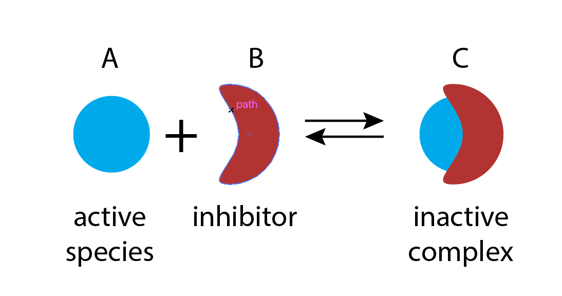
Molecular titration: a minimal model
To see how molecular titration produces ultrasensitivity consider two proteins, A and B, that can bind to form a complex, C, which is inactive for both A and B activities. This system can be described by the following reaction.
\begin{align} \require{mhchem} \ce{A + B <=>[k_\mathrm{on}][k_\mathrm{off}] C}. \end{align}
At steady-state, from mass action kinetics, we have
\begin{align} k_\mathrm{on} a b = k_\mathrm{off} c, \end{align}
where we are using our convention that lowercase symbols denote concentrations of species (e.g., \(a\) is the concentration of A).
Using \(K_\mathrm{d} = k_\mathrm{off}/k_\mathrm{on}\), we can write this as
\begin{align} a b = K_\mathrm{d} c. \end{align}
We also will insist on conservation of mass,
\begin{align} a_\mathrm{tot} &= a + c \\[1em] b_\mathrm{tot} &= b + c. \end{align}
Here, \(a_\mathrm{tot}\) and \(b_\mathrm{tot}\) denote the total amounts of A and B, respectively. We can solve the three equations for the three unknowns, the concentrations of A, B, and C. The solution provides an expression for the amount of free A or free B as a function of \(a_\mathrm{tot}\) and \(b_\mathrm{tot}\) for different values of \(K_\mathrm{d}\).
\begin{align} a = \frac{1}{2} \left(a_\mathrm{tot} - b_\mathrm{tot} - K_\mathrm{d} + \sqrt{ (a_\mathrm{tot} - b_\mathrm{tot} - K_\mathrm{d})^2 + 4 a_\mathrm{tot} K_\mathrm{d}}\right). \end{align}
What does this relationship look like? Let’s consider a case in which we control the total amount of \(a_\mathrm{tot}\) and see how much free A we get, for different amounts of \(b_\mathrm{tot}\). We will start by assuming the limit of strong binding (small values of \(K_\mathrm{d}\), taking \(K_\mathrm{d} = 10\) nM), plotting the amount of free A on both linear and log-log scales.
[5]:
def free_a(a_tot, b_tot, Kd):
    discrim = (a_tot - b_tot - Kd) ** 2 + 4 * a_tot * Kd
    return (a_tot - b_tot - Kd + np.sqrt(discrim)) / 2


a_tot = np.linspace(0, 200, 1001)
Kd = 0.001
b_tot_vals = np.array([50, 100, 150])

colors = bokeh.palettes.Blues3

p = bokeh.plotting.figure(
    width=450,
    height=300,
    x_axis_label="total A conc. (µM)",
    y_axis_label="free A conc. (µM)",
    x_range=[a_tot.min(), a_tot.max()],
    title="Strong binding regime",
)

for i, (color, b_tot) in enumerate(zip(colors, b_tot_vals)):
    a = free_a(a_tot, b_tot, Kd)
    p.line(a_tot, a, line_width=2, color=color, legend_label=str(b_tot) + " µM")

p.legend.location = "top_left"
p.legend.title = "total B conc."
bokeh.io.show(p)
In these curves, we see that when \(a_\mathrm{tot} < b_\mathrm{tot}\), A is completely sequestered by B, and therefore close to 0. When \(a_\mathrm{tot} > b_\mathrm{tot}\), it rises linearly, becoming approximately proportional to the difference \(a_\mathrm{tot} - b_\mathrm{tot}\). This is called a threshold-linear relationship. Plotting the same relationship on a log-log scale is also informative:
[6]:
a_tot = np.logspace(-2, 6, 1001)
b_tot_vals = np.logspace(-1, 3, 5)

colors = bokeh.palettes.Blues9[3:8]

p = bokeh.plotting.figure(
    width=450,
    height=300,
    x_axis_label="total A conc. (µM)",
    y_axis_label="free A conc. (µM)",
    x_axis_type="log",
    y_axis_type="log",
    x_range=[a_tot.min(), a_tot.max()],
    title="Strong binding regime",
)

for i, (color, b_tot) in enumerate(zip(colors, b_tot_vals)):
    a = free_a(a_tot, b_tot, Kd)
    p.line(a_tot, a, line_width=2, color=color, legend_label=str(b_tot)+" µM")

p.legend.location = "bottom_right"
p.legend.title = "total B conc."

bokeh.io.show(p)
The key feature to notice here is that A accumulates linearly at low and high values of \(a_\mathrm{tot}\), but in between goes through a sharp transition, with a much higher slope, indicating ultrasensitivity, around \(b_\mathrm{tot}\).
So far, we have looked in the strong binding limit, that is the regime with very slow unbinding and therefore small \(K_\mathrm{d}\). Any real system will have a finite rate of unbinding. It is therefore important to see how the system behaves across a range of \(K_\mathrm{d}\) values. To investigate this, we fix \(b = 1\) µM and make a plot of free versus total A for various values of \(K_\mathrm{d}\).
[7]:
a_tot = np.logspace(-2, 3, 1001)
b_tot = 1
Kd_vals = np.logspace(-3, 1, 5)

colors = bokeh.palettes.Blues9[3:8]

p = bokeh.plotting.figure(
    width=450,
    height=300,
    x_axis_label="total A conc. (µM)",
    y_axis_label="free A conc. (µM)",
    x_axis_type="log",
    y_axis_type="log",
    x_range=[a_tot.min(), a_tot.max()],
)

for i, (color, Kd) in enumerate(zip(colors, Kd_vals)):
    a = free_a(a_tot, b_tot, Kd)
    p.line(a_tot, a, line_width=2, color=color, legend_label=str(Kd)+" µM")

p.legend.location = "bottom_right"
p.legend.title = "Kd"

bokeh.io.show(p)
Here we see that the tighter the binding, the more completely B shuts off A, and the larger the region of ultrasensitivity around the transition point. On a linear scale, zooming in around the transition point, we can see that weaker binding “softens” the transition from flat to linear behavior:
[8]:
a_tot = np.linspace(0, 2, 1001)

p = bokeh.plotting.figure(
    width=450,
    height=300,
    x_axis_label="total A conc. (µM)",
    y_axis_label="free A conc. (µM)",
    x_range=[a_tot.min(), a_tot.max()],
)

for i, (color, Kd) in enumerate(zip(colors, Kd_vals)):
    a = free_a(a_tot, b_tot, Kd)
    p.line(a_tot, a, line_width=2, color=color, legend_label=str(Kd)+" µM")

p.legend.location = "top_left"
p.legend.title = "Kd"

bokeh.io.show(p)
Ultrasensitivity in threshold-linear response functions
Threshold-linear responses differ qualitatively from what we had with a Hill function. Unlike the sigmoidal, or “S-shaped,” Hill function, which saturates at a maximum “ceiling,” the threshold-linear function increases without bound, maintaining a constant slope as input values increase.
Despite these differences, we can still quantify the sensitivity of this response, which as a reminder is defined as the fold change in output for a given fold change in input, evaluated at a particular operating point. The plots below show this sensitivity plotted for varying \(a_\mathrm{tot}\), and for different values of \(K_\mathrm{d}\). Note the peak in sensitivity right around the transition, whose strength grows with tighter binding (lower \(K_\mathrm{d}\)). This peak highlights what we see in the input-output function: Ultrasensitivity can be very strong for tight binding (small \(K_\mathrm{d}\)) when \(a_\mathrm{tot} \approx b_\mathrm{tot}\).
[9]:
bokeh.io.show(biocircuits.jsplots.simple_binding_sensitivity())
A synthetic demonstration of molecular titration
Simple models like the ones above can help us think about what behaviors we should expect in a system. But how do we know if they accurately describe the real behavior of a complex molecular system, particularly one operating in the more complex milieu of the living cell? In the spirit of building-to-understand, Buchler and Cross used a synthetic biology approach to investigate how this simple scheme could indeed generate the predicted ultrasensitivity.
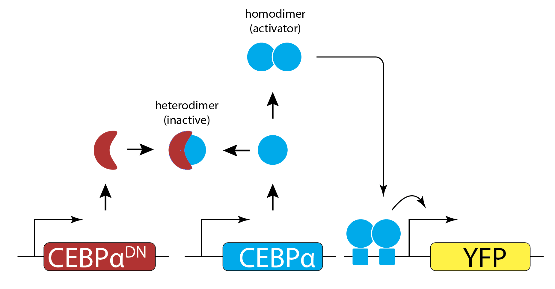
They engineered yeast cells to express a transcription factor, a stoichiometric inhibitor of that factor, and a target reporter gene to readout the level of the transcription factor. As a transcription factor, they used the mammalian bZip family activator CEBP/\(\alpha\), which homodimerizes to activate target genes, and does not exist in yeast. As the inhibitor, they used a dominant negative mutant of CEBP/\(\alpha\) that binds to it with a tight \(K_\mathrm{d} \approx 0.04\) nM to form an inactive complex. As a reporter, they used yellow fluorescent protein expressed from a CEBAα-dependent promoter. To vary the relative levels of the activator and inhibitor, they expressed each of them from a set of distinct promoters of different strengths. The entire circuit was integrated in the yeast genome. As a control, they also constructed yeast strains without the inhibitor.
The scheme is shown here (redrawn from their paper):
Expressing the activator from a series of promoters of different strengths, without the inhibitor, generated a dose-dependent increase in the fluorescent protein, as expected. (You will also notice a decrease at the highest levels of activator expression. They attributed this decline to a phenomenon known as transcriptional “squelching” in which extremely high expression of a transcriptional activator can tie up core transcriptional components, such as RNA polymerase, reducing their ability to activate other genes.)
By contrast, when they also expressed the inhibitor at a fixed concentration, \(b_\mathrm{tot}\) (middle panel), they observed no induction of YFP for concentrations of CEBPα lower than \(b_\mathrm{tot}\). When CEBPα level exceeded \(b_\mathrm{tot}\), however, YFP levels rapidly increased. This threshold linear response resembled those predicted in the model. (Squelching can be observed in this plot as well.)
Finally, expressing the inhibitor from promoters of different strengths (right) produced corresponding shifts in the threshold position, as expected based on their independently measured expression level (colored arrows).
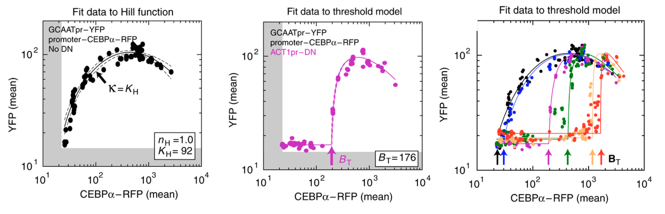
Figure fromBuchler and Cross
These results show that the circuit feature of molecular titration can be reconstituted and quantitatively predicted in living cells, and can generate ultrasensitive responses with a tunable threshold.
We now turn to non-engineered contexts in which molecular titration appears.
Small RNA regulation can generate ultrasensitive responses through molecular titration
The last few decades have revealed different classes of RNA molecules that play a wide range of regulatory roles within the cell. In particular, small RNA molecules regulate gene expression in systems from bacteria to mammalian cells. microRNA (miRNA) represents a major class of regulatory RNA molecules in eukaryotes. Humans have hundreds of miRNAs, with individual miRNAs typically targeting hundreds of genes. 30-90% of human protein-coding genes are targets of one or more miRNAs. Individual miRNAs can also be highly expressed (as many as 50,000 copies per cell in C. elegans). Many miRNAs exhibit strong sequence conservation across species, suggesting selection for function.
Confusingly, however, at the cell population average level, they sometimes appear to generate relatively weak repression. To more quantitatively understand how miRNA regulation operates, Mukherji et al developed a system to analyze miRNA regulation at the level of single cells (Mukherji, S., et al, Nat. Methods, 2011).
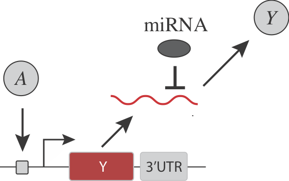
To analyze the magnitude of miRNA regulation, they expressed two different colored fluorescent proteins, one regulated by a specific miRNA, the other serving as an unregulated internal control. This design allows one to visualize and quantify the magnitude of miRNA regulation in individual cell.
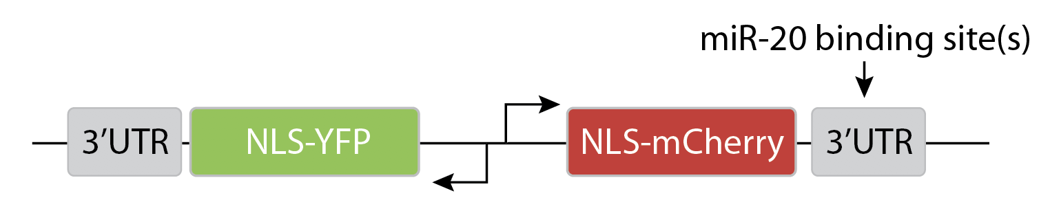
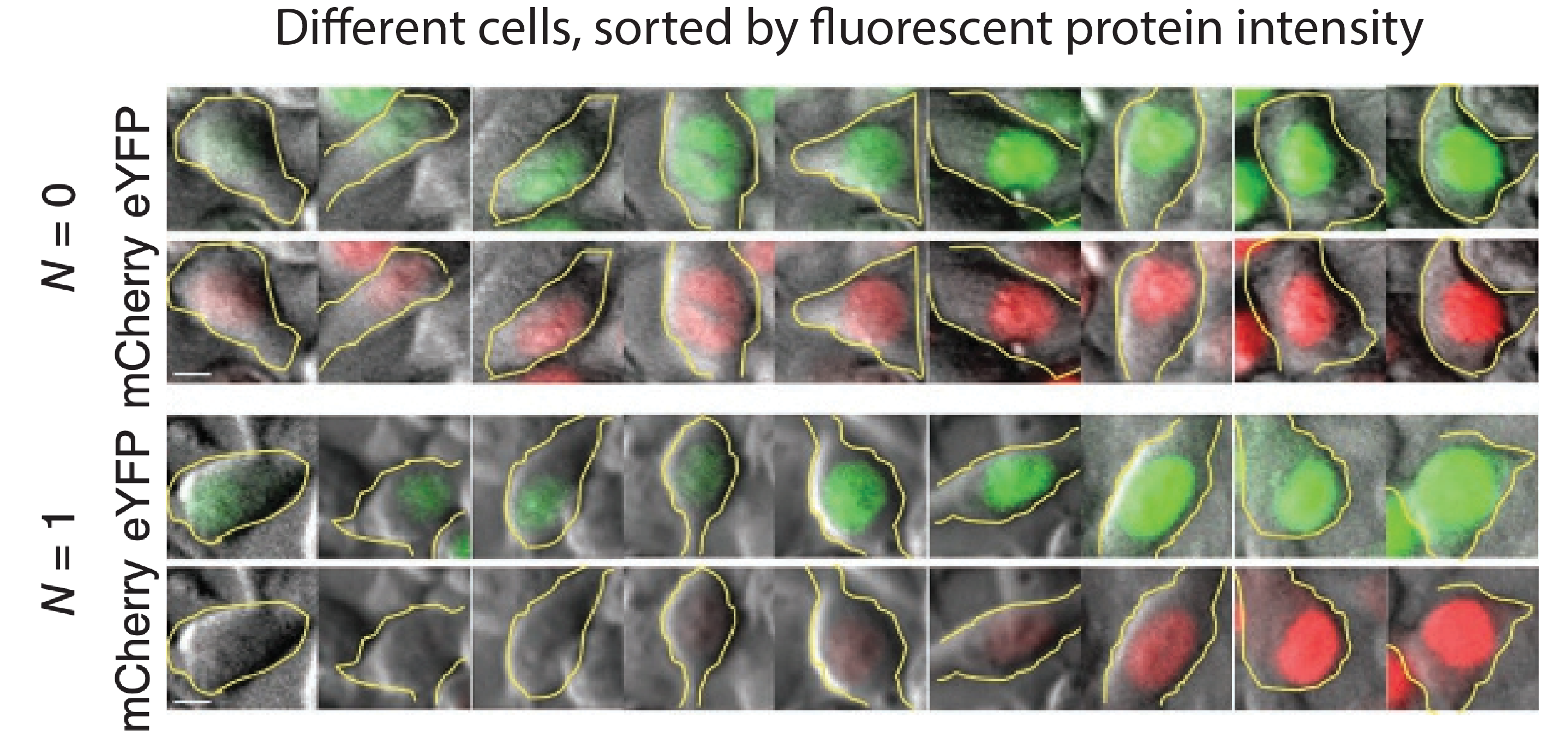
They transfected variants of this construct with (N=1) or without (N=0) a binding site for the miR-20 miRNA. The images below show the levels of the two proteins in different individual cells, sorted by their intensity. The top pair of rows shows the case with no miRNA binding sites, and the lower pair of rows shows the case with binding sites. Without the binding site, the two colors appear to be proportional to each other, as you would expect, since they are co-regulated. On the other hand, with the binding site, mCherry expression is suppressed at lower YFP expression levels. Only at the higher YFP levels do you start to see the mCherry signal growing. This looks like the kind of threshold-linear response one expects from molecular titration.
Indeed, threshold-linear behavior can be seen more clearly in a scatter plot of the two colors:
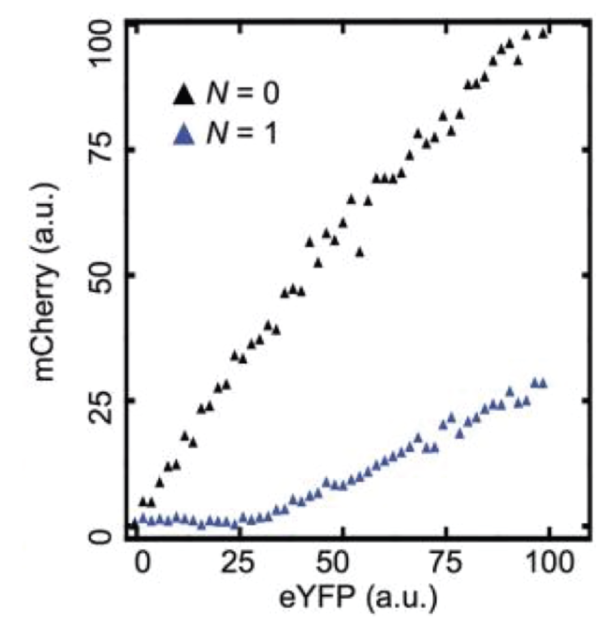
Here, the YFP x-axis is analogous to our \(a_\mathrm{tot}\), above, while the mCherry y-axis is analogous to \(a\).
Modeling the miRNA system
So far, we considered a static pool of A and B, but in a cell, both proteins undergo continuous synthesis as well as degradation and/or dilution. To explain the miRNA system, several papers, including Mukherji, et al., 2011, as well as Buchler & Louis, 2008, Levine, et al., 2007, and Mehta, et al., 2008 use similar representations. The following analysis follows the treatment in the supplementary material of Mukherji, et al., but with altered notation.
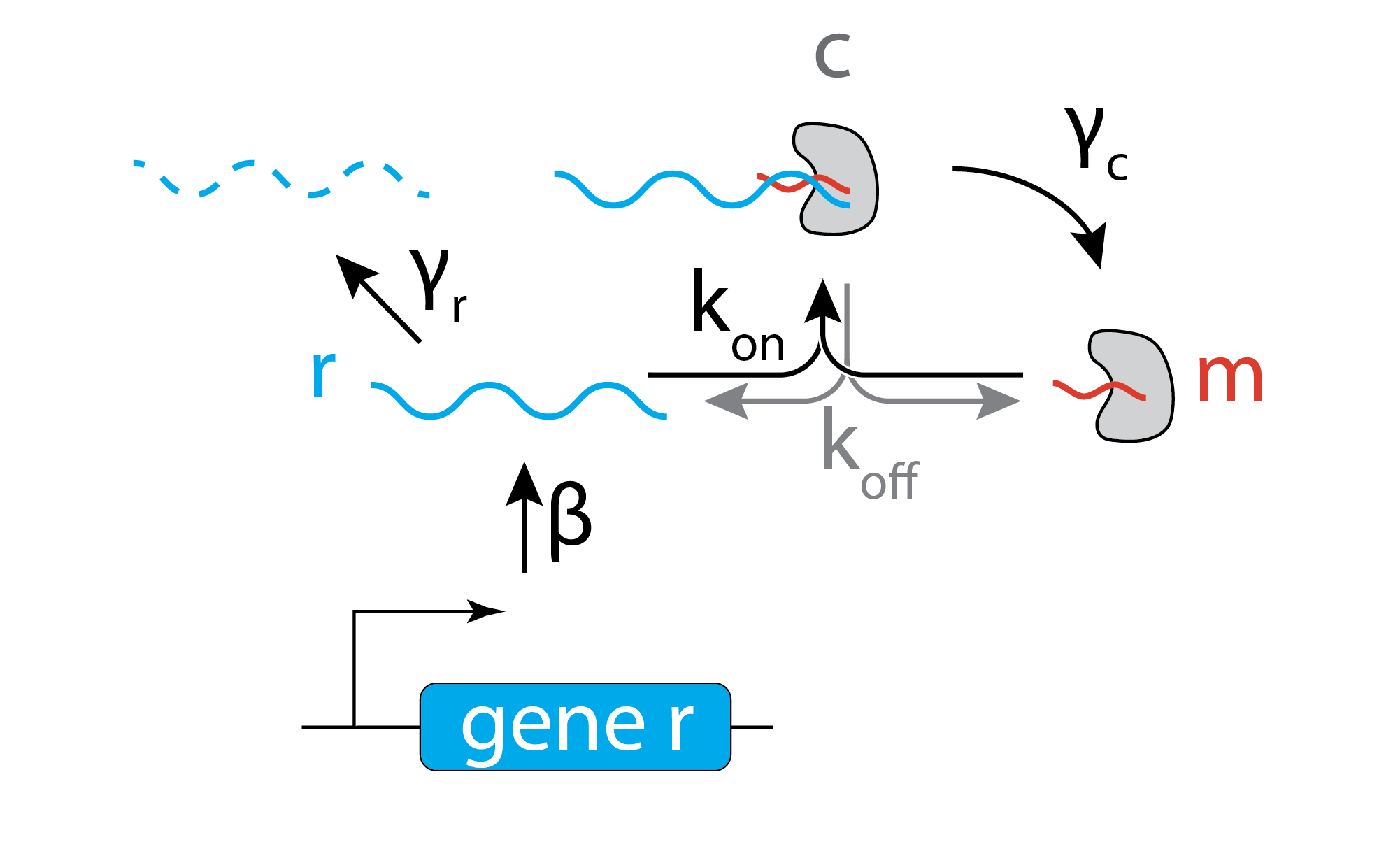
For simplicity, we assume that the target mRNA, denoted \(r\) is produced at a constant rate, \(\beta\), and degraded at rate \(\gamma_r\). It can bind to a miRNA, denoted \(m\), at a rate \(k_\mathrm{on} r m\) to form a complex, \(c\), and unbinds at a rate \(k_\mathrm{off} c\). The complex itself can degrade with rate constant \(\gamma_c\), destroying the target mRNA, but leaving the miRNA intact. This model thus assumes the miRNA acts catalytically, with a single miRNA (or, really, its RISC complex) potentially destroying multiple mRNA molecules. We therefore assume that the total amount of miRNA is a constant, \(m_\mathrm{tot}\).
\begin{align} &\frac{\mathrm{dr}}{\mathrm{d}t} = - k_\mathrm{on} r m + k_\mathrm{off} c - \gamma_r r + \beta \\[1em] &\frac{\mathrm{dc}}{\mathrm{d}t} = k_\mathrm{on} r m - k_\mathrm{off} c - \gamma_c c \\[1em] &m_{\mathrm{tot}} = c + m \end{align}
Focusing on the steady-state, as usual, we set the time derivatives to 0 and solve for \(r\), which represents the free mRNA, which will be translated to produce protein, and hence is our proxy for the output of the system.
We will further define a few natural parameters combinations: - \(r_0 = \beta / \gamma_r\) is the unregulated steady state expression of r - \(\lambda = \frac{\gamma_c + k_\mathrm{off}}{k_\mathrm{on}}\) represents the “tightness” of the interaction. Small values of \(\lambda\) indicate that complexes are formed faster than they can degrade or fall apart. - \(\theta = m_\mathrm{tot} \frac{\gamma_c}{\gamma_r}\) represents the impact of the miRNA. If the miRNA concentration, \(m_\mathrm{tot}\), is large and if it generates a complex that degrades rapidly compared to the spontaneous degradation of the mRNA, then it will have a strong impact on the target mRNA.
Adding the first two equations together gives one relationship between \(r\) and \(c\), \(\beta - \gamma_r r - \gamma_c c = 0\), which can be rearranged to give
\begin{align} c = \frac{\beta-\gamma_r r}{\gamma_c} \end{align}
Then we can take the \(\mathrm{d}c/\mathrm{d}t = 0\) equation and solve for \(c\) as a function of \(r\),
\begin{align} c = \frac{k_\mathrm{on}\,m_\mathrm{tot}\,r}{k_\mathrm{on}\,r + k_\mathrm{off} + \gamma_c}. \end{align}
Setting these two equations equal to each other gives us a single quadratic equation for \(r\), using the definitions above,
\begin{align} r^2 + r (\lambda + \theta - r_0) - \lambda r_0 = 0. \end{align}
The solution is
\begin{align} r = \frac{1}{2} \left(r_0 - \lambda - \theta + \sqrt{(\lambda + \theta - r_0)^2 + 4 \lambda r_0}\right) \end{align}
Let’s see how this expression behaves in different regimes.
[10]:
def rna_level(r0, lam, theta):
    b = r0 - lam - theta
    return (b + np.sqrt(b ** 2 + 4 * lam * r0)) / 2


r0_lin = np.linspace(0, 4, 400)
r0_log = np.logspace(-2, 2, 400)
theta = np.logspace(-1, 1, 5)
lam = np.logspace(-2, 2, 5)

theta_labels = [0.1, 0.3, 1, 3, 10]
colors = bokeh.palettes.Blues8

p_lam_lin = bokeh.plotting.figure(
    frame_width=270,
    frame_height=270,
    x_axis_label="r₀",
    y_axis_label="r",
    x_range=[r0_lin.min(), r0_lin.max()],
    title="θ = 1",
)

for i, lam_ in enumerate(lam):
    p_lam_lin.line(
        r0_lin,
        rna_level(r0_lin, lam_, theta[len(theta) // 2]),
        line_width=2,
        color=colors[i],
        legend_label=f"λ = {lam_}",
    )

p_lam_lin.legend.location = "top_left"

p_lam_log = bokeh.plotting.figure(
    frame_width=270,
    frame_height=270,
    x_axis_label="r₀",
    y_axis_label="r",
    x_range=[r0_log.min(), r0_log.max()],
    y_range=[1e-4, 1e2],
    x_axis_type="log",
    y_axis_type="log",
    title="θ = 1",
)

for i, lam_ in enumerate(lam):
    p_lam_log.line(
        r0_log,
        rna_level(r0_log, lam_, theta[len(theta) // 2]),
        line_width=2,
        color=colors[i],
        legend_label=f"λ = {lam_}",
    )

p_lam_log.legend.location = "top_left"
p_lam_log.visible = False
p_lam_lin.visible = True

radio_button_group = bokeh.models.RadioButtonGroup(
    labels=["log", "linear"], active=1, width=100
)

col_lam = bokeh.layouts.column(
    p_lam_lin,
    p_lam_log,
    bokeh.layouts.row(bokeh.models.Spacer(width=100), radio_button_group),
)

radio_button_group.js_on_click(
    bokeh.models.CustomJS(
        args=dict(p_lam_log=p_lam_log, p_lam_lin=p_lam_lin),
        code="""
  if (p_lam_log.visible == true) {
    p_lam_log.visible = false;
    p_lam_lin.visible = true;
  }
  else {
    p_lam_log.visible = true;
    p_lam_lin.visible = false;
  }
""",
    )
)

for i, lam_ in enumerate(lam):
    p_lam_lin.line(
        r0_lin,
        rna_level(r0_lin, lam_, theta[len(theta) // 2]),
        line_width=2,
        color=colors[i],
        legend_label=f"λ = {lam_}",
    )

p_lam_lin.legend.location = "top_left"

p_theta_lin = bokeh.plotting.figure(
    frame_width=270,
    frame_height=270,
    x_axis_label="r₀",
    y_axis_label="r",
    x_range=[r0_lin.min(), r0_lin.max()],
    title="λ = 1",
)

for i, theta_ in enumerate(theta):
    p_theta_lin.line(
        r0_lin,
        rna_level(r0_lin, lam[len(lam) // 2], theta_),
        line_width=2,
        color=colors[i],
        legend_label=f"θ = {theta_labels[i]}",
    )
p_theta_lin.legend.location = "top_left"

p_theta_log = bokeh.plotting.figure(
    frame_width=270,
    frame_height=270,
    x_axis_label="r₀",
    y_axis_label="r",
    x_range=[r0_log.min(), r0_log.max()],
    y_range=[7e-4, 1e2],
    x_axis_type="log",
    y_axis_type="log",
    title="λ = 1",
)

for i, theta_ in enumerate(theta):
    p_theta_log.line(
        r0_log,
        rna_level(r0_log, theta_, theta[len(theta) // 2]),
        line_width=2,
        color=colors[i],
        legend_label=f"θ = {theta_labels[i]}",
    )
p_theta_log.legend.location = "top_left"
p_theta_log.visible = False
p_theta_lin.visible = True

radio_button_group = bokeh.models.RadioButtonGroup(
    labels=["log", "linear"], active=1, width=100
)

col_theta = bokeh.layouts.column(
    p_theta_lin,
    p_theta_log,
    bokeh.layouts.row(bokeh.models.Spacer(width=100), radio_button_group),
)

radio_button_group.js_on_click(
    bokeh.models.CustomJS(
        args=dict(p_theta_log=p_theta_log, p_theta_lin=p_theta_lin),
        code="""
  if (p_theta_log.visible == true) {
    p_theta_log.visible = false;
    p_theta_lin.visible = true;
  }
  else {
    p_theta_log.visible = true;
    p_theta_lin.visible = false;
  }
""",
    )
)

bokeh.io.show(bokeh.layouts.row([col_lam, col_theta]))
On the left plot, we can see that decreasing \(\lambda\), which is equivalent to increasing \(k_{\mathrm{on}}\), or strengthening the miRNA-mRNA interaction, makes the response increasingly threshold-linear. On the right, we see that increasing \(\theta\), which is equivalent to increasing total miRNA concentration, extends the suppression regime to higher values of \(r_0\). Also notice that it can generate reduced slopes for the \(r\) versus \(r_0\) response function, similar to those observed in the experimental data shown above.
The authors go on to explore how increasing the number of binding sites can modulate the threshold for repression and show that the experimental results broadly fit the behavior expected from the molecular titration model.
These results could help reconcile the very different types of effects one sees for miRNAs in different contexts. Sometimes they appear to provide strong, switch-like effects, as with fate-controlling miRNAs in C. elegans. On the other hand, in many other contexts, they appear to exert much weaker “fine-tuning” effects on their targets.
That makes sense: when miRNAs are unsaturated, they can have a relatively strong effect on their target expression levels, essentially keeping them “off.” On the other hand, when targets are expressed highly enough, the relative effect of the miRNA on expression becomes much weaker, effectively just shifting it to slightly slower values.
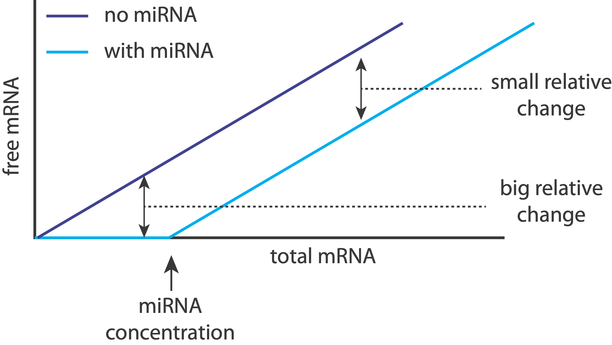
Returning to the question posed earlier, we now see that inserting a constitutive, inhibitory miRNA provides an elegant way to threshold a gene regulatory interaction.
Note that in addition to its general regulatory abilities and thresholding effects, miRNA regulation can also reduce noise in target gene expression. See Schmiedel et al, “MicroRNA control of protein expression noise,” Science (2015).
Molecular titration in antibiotic persistence
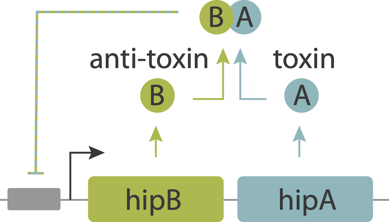
In an upcoming chapter, we will analyze a phenomenon known as antibiotic persistence, in which individual bacteria spontaneously and stochastically enter slow-growing persistent states that tolerate antibiotics, even in the absence of those antibiotics. One such system in E. coli is controlled by the hipAB circuit, which comprises a toxin protein, HipA, and a cognate anti-toxin, HipB. The two proteins are expressed from a single operon. They form tight complexes that also act to repress their own promoter. If the levels of the HipA toxin exceed those of the HipB anti-toxin, for example due to stochastic fluctuations in expession, it can trigger a transition into the persistent state.
Evidence that molecular titration plays a key role in activation of persistence was shown by Rotem et al. Among many experiments, they created a partial open loop strain in which they could independently control hipA and read its level out in individual cells using a co-transcribed red fluorescent protein (mCherry):
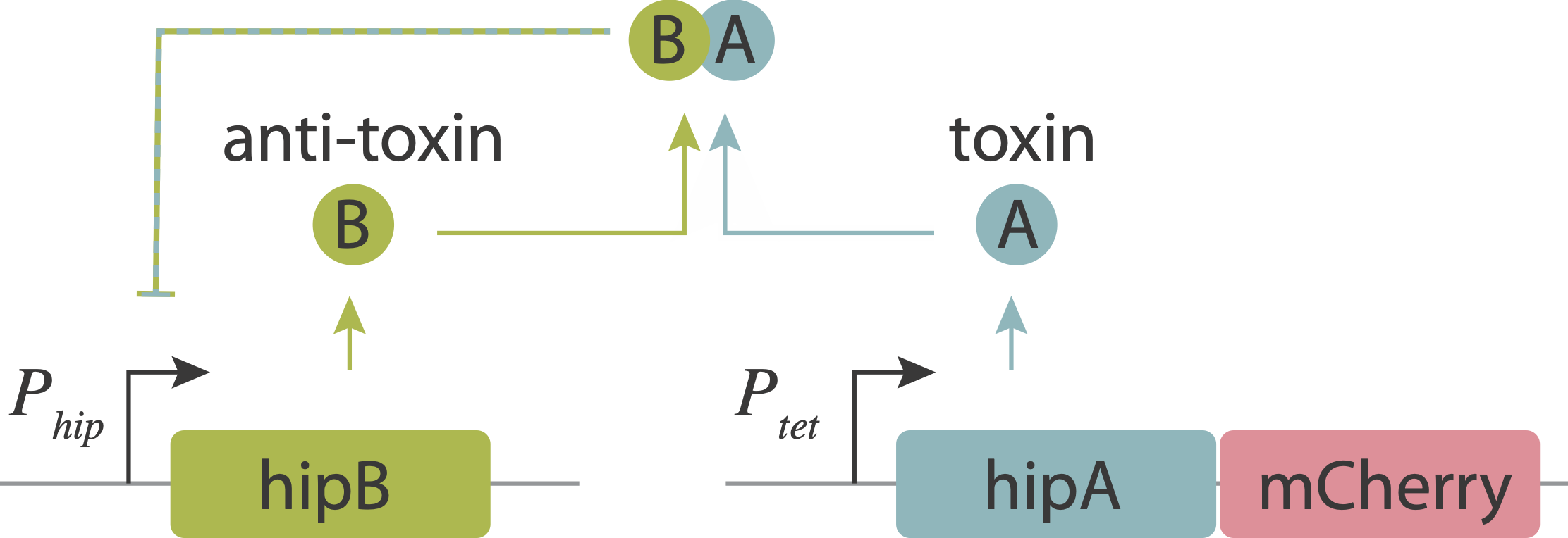
They then used time-lapse movies to correlate the growth behavior of individual cells with their HipA protein levels. As shown in these panels, cells with higher levels of mCherry showed delayed growth. Analyzing these data quantitatively revealed (drumroll, please) a threshold relationship, in which growth arrest occurred when HipA (as measured by its fluorescent protein tag) exceeded a threshold concentration:
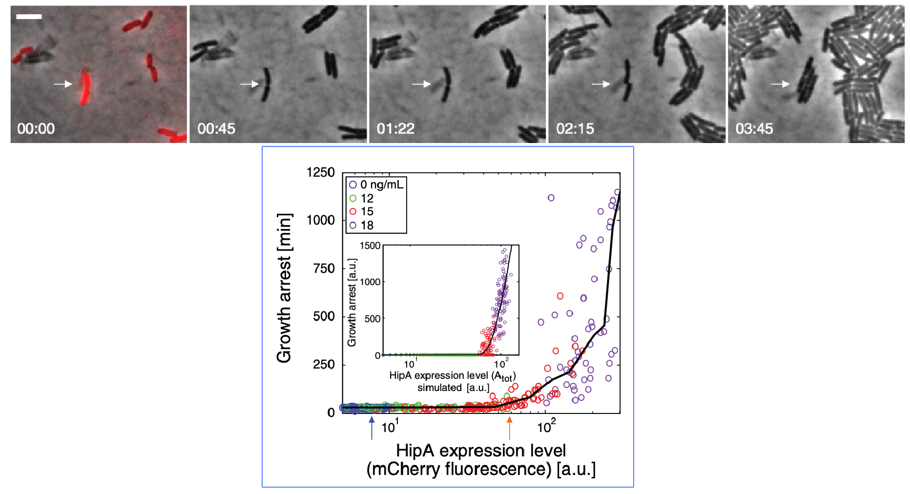
Note that the inset in the plot is the behavior of a mathematical model of the circuit.
We will come back to this circuit later once we have the tools to analyze and simulate noise, and understand how noise combines with molecular titration to enable this important phenomenon.
Beyond pairwise titration
Today we talked about molecular titration arising from interactions between protein pairs. However, proteins often form more complex, and even combinatorial, networks of homo- and hetero-dimerizing components. One example occurs in the control of cell death (apoptosis) by Bcl2-family proteins, a process that naturally should be performed in an all-or-none way. In the next chapter, we will learn about a synthetic circuit that takes advantage of these interactions to generate multistability in mammalian cells.
Conclusions
Today we have seen that molecular titration provides a powerful, elegant way to generate ultrasensitive responses across different types of molecular systems:
The general principle of molecular titration: formation of a tight complex between two species makes the concentration of a “free” protein species depend in a threshold-linear manner on its total level or rate of production.
Molecular titration can be observed in synthetic experiments.
Molecular titration explains some features of miRNA based regulation and could underlie the generation of bacterial persisters through toxin-antitoxin systems.
References
Molecular titration can generate ultrasensitive switches:
Ferrell JE Jr and Ha SH wrote a three-part series of articles on ultrasensitivity: Part I, Part II, and Part III are all excellent, but part II in particular covers stoichiometric inhibitors, which is the main focus of this chapter.
N.E. Buchler and F.R. Cross, Protein sequestration generates a flexible ultrasensitive response in a genetic network, Mol. Syst. Biol. (2009).
Kim J, White KS, and Winfree E, Construction of an in vitro bistable circuit from synthetic transcriptional switches, Molecular Systems Biology (2006).
Cuba Samaniego C et al, Molecular Titration Promotes Oscillations and Bistability in Minimal Network Models with Monomeric Regulators, ACS Synthetic Biology (2016).
Molecular titration in regulation by small RNAs:
Molecular titration antibiotic persistence:
Computing environment
[11]:
%load_ext watermark
%watermark -v -p numpy,biocircuits,bokeh,jupyterlab
Python implementation: CPython
Python version       : 3.9.12
IPython version      : 8.2.0

numpy      : 1.21.5
biocircuits: 0.1.8
bokeh      : 2.4.2
jupyterlab : 3.3.2