18. Excitability enables probabilistic, transient differentiation
Design principles
Fast positive feedback combined with slow negative feedback can combine to give excitable circuits.
Excitability enables probabilistic, transient differentiation
Concepts
Excitable circuits have a unique, globally attracting rest state and a large stimulus can send the system on a long excursion before it returns to the resting state.
[30]:
# Colab setup ------------------
import os, sys, subprocess
if "google.colab" in sys.modules:
    cmd = "pip install --upgrade biocircuits iqplot numba multiprocess watermark"
    process = subprocess.Popen(cmd.split(), stdout=subprocess.PIPE, stderr=subprocess.PIPE)
    stdout, stderr = process.communicate()
# ------------------------------

import collections
import tqdm

import pandas as pd
import numpy as np
import scipy.integrate
import numba

import biocircuits

import bokeh.io
import bokeh.plotting

import iqplot

# Toggle for fully interactive plots
fully_interactive_plots = True
notebook_url = "localhost:8888"

bokeh.io.output_notebook()
Altered states
Cells can exist in a broad repertoire of physiologically distinct states with different properties. In the previous chapter we saw how spontaneous transitions to slow growing states can give rise to antibiotic persistence in bacteria, effectively sacrificing the growth of some cells to increase the survival probability of their clone. In fact, cells are constantly switching in and out of a myriad of different physiological states.
We have now encountered several different features of dynamical systems that each enable a distinct cellular capability:
Dynamical system property |
Cellular capability |
|---|---|
Monostable fixed point |
Remain in a constant state (homeostasis) |
Bistability / multistability |
Exist in two or more epigenetically stable states (e.g., toggle switch, MultiFate) |
Limit cycles |
Periodic oscillations (e.g., repressilator) |
In this chapter, we will add a new line to this table, showing how excitability takes advantage of noise to probabilistically initiate transient episodes of differentiation. Furthermore, we will see how the circuit architecture makes it possible for bacteria to independently modulate two key properties of these episodes: their frequency and their duration. We will discuss excitability in the context of cellular competence.
Excitability is tricky to define. Borrowing from Strogatz (in Nonlinear Dynamics and Chaos) an excitable system has two key properties:
It has a unique, globally attracting rest state;
A large enough stimulus can send the system on a long excursion before it returns to the resting state.
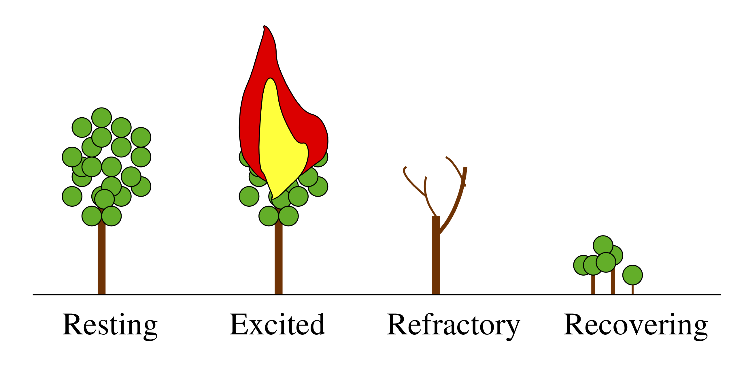
Excitability is prevalent
A forest is a classic example of an excitable system. Its resting state consists of many trees peacefully photosynthesizing and providing shade for hikers. Occasionally, though, a relatively small perturbation, perhaps an errant lightning strike or a careless camper, can dramatically alter the landscape, initiating a transient excursion wherein the forest burns, recovers, and then grows back again.
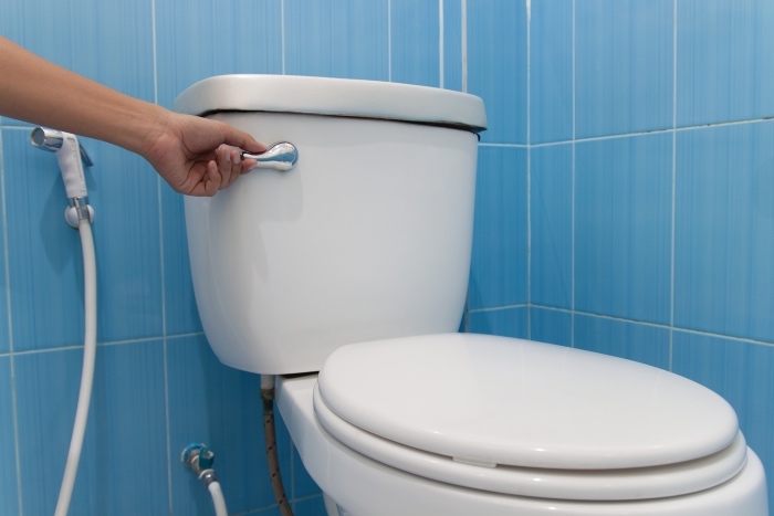
The most familiar example of excitability may be a toilet. Normally the toilet sits at rest in a more or less constant state. Pressing the handle strongly enough initiates a stereotyped sequence of events: the bowl drains, refills with water, and returns to its initial resting state. This is a deterministic system. But imagine adding noise by jiggling the handle. Most of the jiggles have no effect. But occasionally one can be strong enough to cross the threshold and initiate a flush. When that happens, the resulting flush cycle is the same as one initiated by a deliberate push. It does not matter how the threshold is crossed. In an excitable system like this, any threshold-crossing perturbation—whether external or from noise—generates a similar dynamic trajectory.
Closer to molecular biology, the membrane potentials of neurons also represent excitable systems. When resting, they sit at their postsynaptic potential (PSP) and a stimulus results in them relaxing immediately back to their PSP. However, when they are excitable, a stimulus can lead to a much larger excursion, called an action potential, or spike, in which the membrane potential grows far beyond the PSP, before returning back to the PSP.
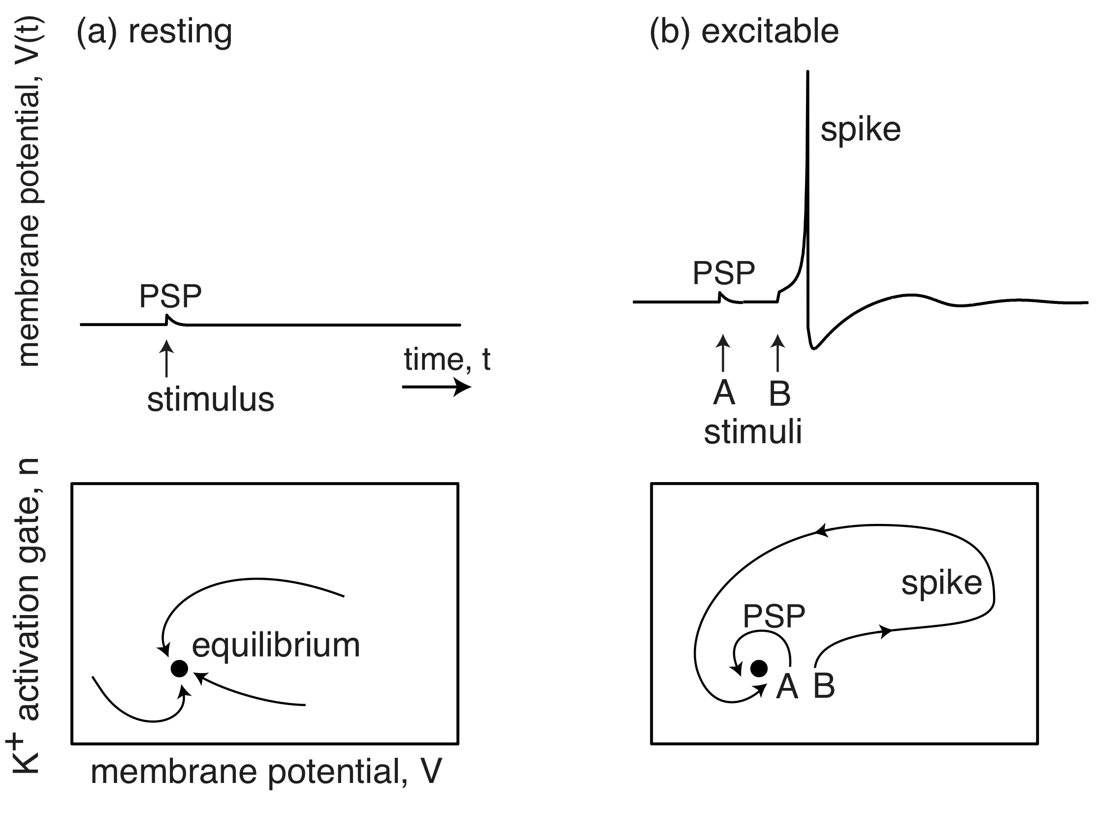
(Image adapted from Izhikevich, Dynamical Systems in Neuroscience, 2007.)
Cellular competence
Now let’s see how bacteria take advantage of excitability. When stressed, some bacteria, such as Bacillus subtilis, can activate a variety of stress response pathways. This activation can be heterogeneous, with different cells activating different responses, even in the same conditions.
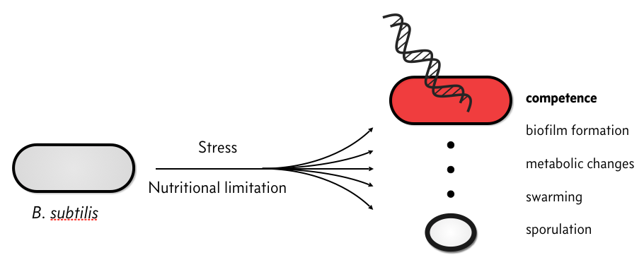
One of these responses is to enter a competent state in which the cell can take up environmental DNA and recombine it into its own genome. This process represents a type of genetic exchange that could provide evolutionary advantages similar to sexual reproduction. But competence also carries risks. The cell might take up viral DNA, for instance. Hence, from a bet hedging point of view, it may be advantageous to activate it in some, but not all, cells within the population.
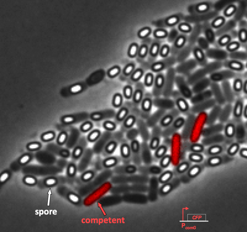
Some of the heterogeneity of stress response can be observed in the following time-lapse movie. In the movie below, cells have been engineered to light up as pink/purple when they become competent. But in the same conditions, cells can also transform into dormant spores, which appear as white ovals in the microscope. So at least two stress responses are clearly evident in the same conditions:
From this movie, it is evident that competence is both probabilistic (only a fraction of cells become competent) and transient (competence is a temporary condition). These are both hallmarks of excitability.
We will now examine the genetic circuit responsible for this excitability and seek to address the following questions:
How do cells enter and exit competence?
How do cells regulate the frequency and duration of competence?
Can these properties be tuned?
Is noise necessary to induce competence?
The B. subtilis competence circuit
The genetic circuit responsible for competence is connected to receptors responsible for sensing the environment and other circuits within the cell. It can appear quite complicated, as shown in the figure below.
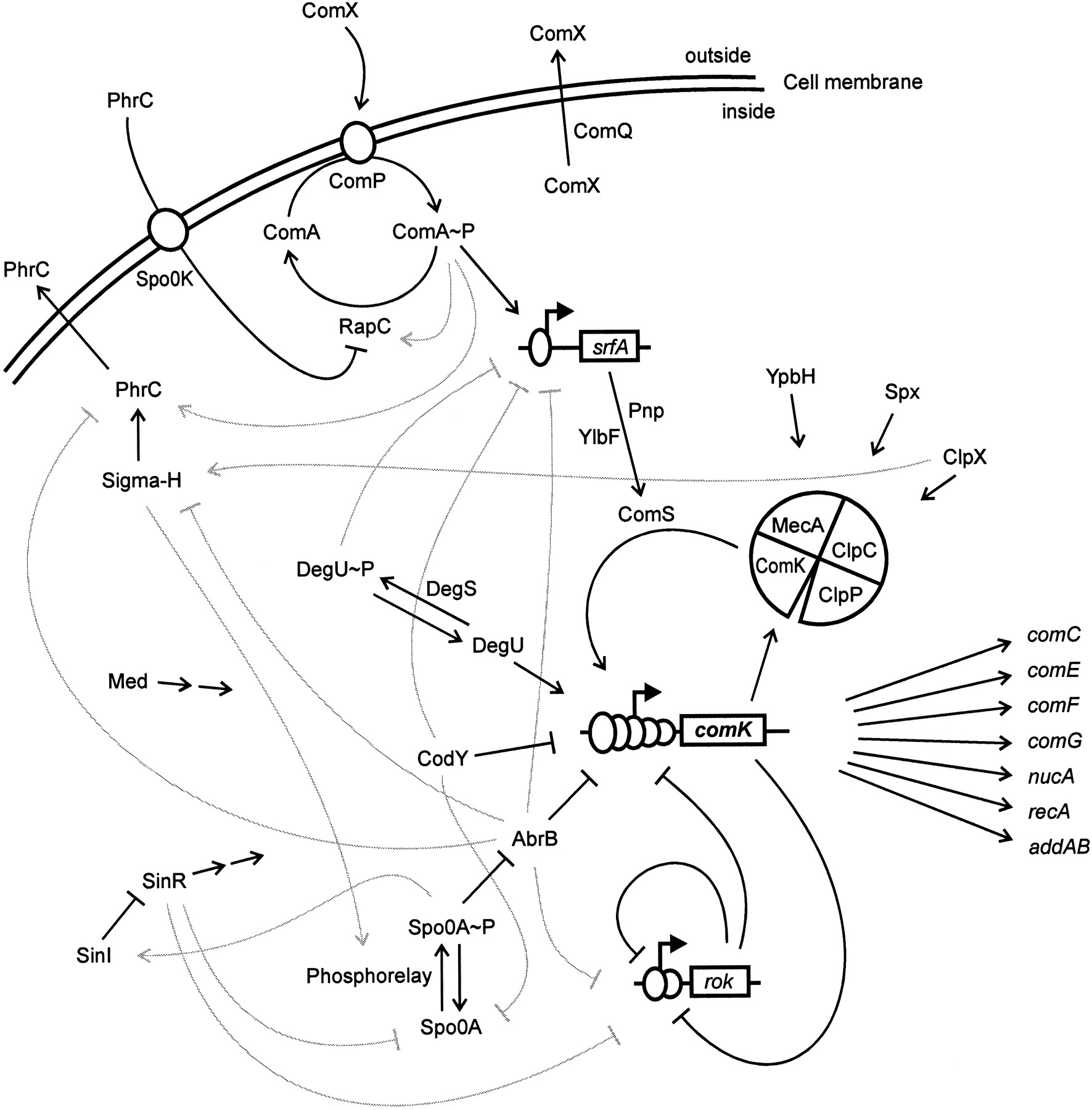
Image taken fromHamoan, et al., Microbiology, 2003
To follow the dynamics of the circuit, Süel, et al. inserted combinations of yellow (YFP) and cyan (CFP) fluorescent reporter genes for various competence genes such as comK, comG and comS in B. subtilis, enabling them to monitor their dynamics in single cells. ComK (blue channel) and ComG (red channel) activate together in competent cells.
Expression of ComK, which has many inputs, largely follows expression of ComG, whose primary input is ComK. (This is why the competent cells appeared purple (blue + red) in the movie above.) This suggested that ComK is the primary regulator of its own expression, at least under these conditions. A second key discovery came from observing ComS and ComG act the same time in two colors. In the movie below, you can see how ComS, in green, declines just as the cell becomes competent (turns on ComK, as shown by the red reporter). This provided compelling evidence for the negative regulatory feedback loop above.
Through these and other experiments, Süel, et al were able to identify a simpler 3-gene core circuit, comprising ComK, ComS, and MecA, that could account for the probabilistic and transient nature of competence differentiation.
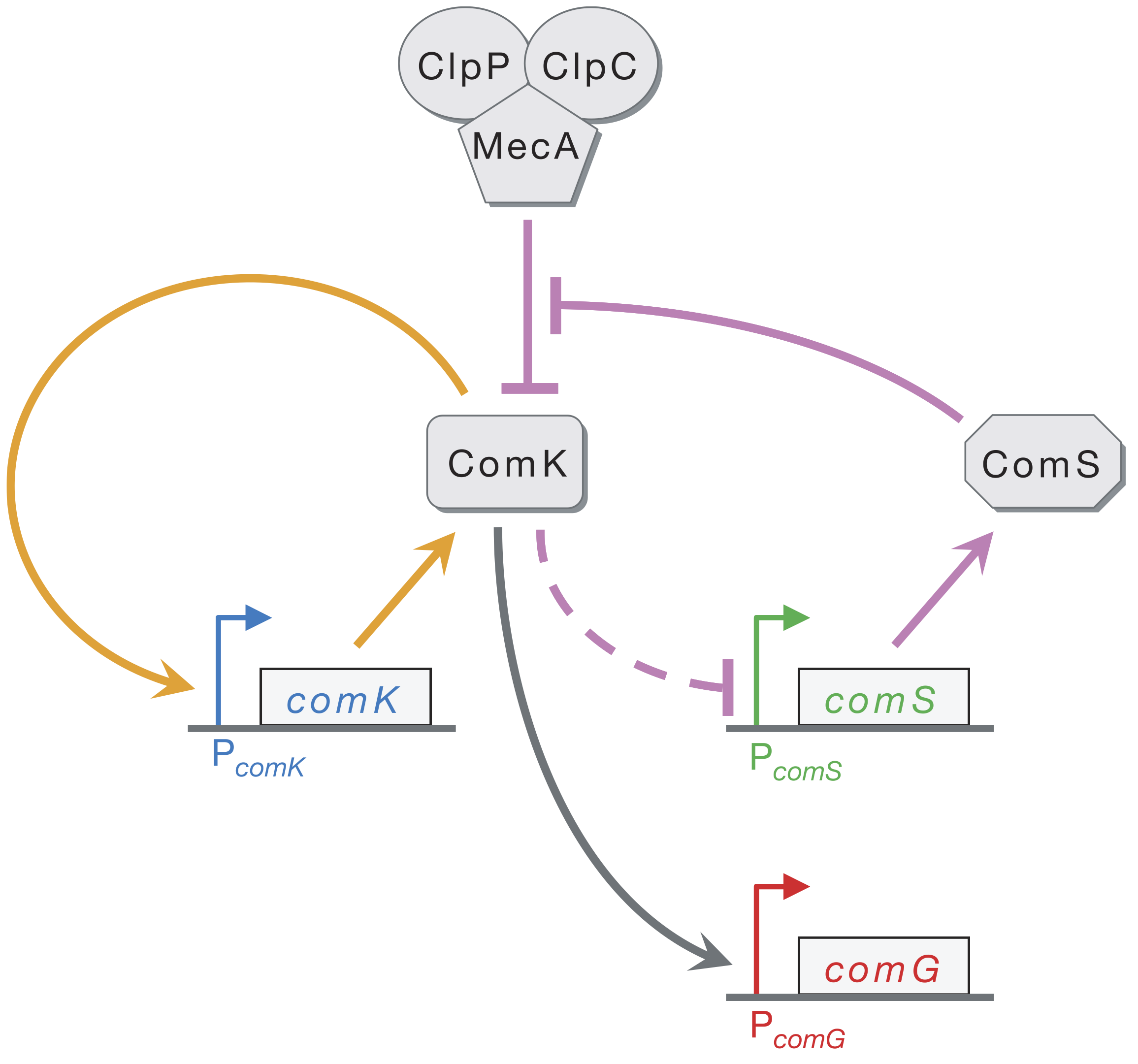
Here, ComK activates its own transcription in a positive feedback loop (orange) and indirectly represses ComS (dashed line). Both ComK and ComS are degraded by the MecA–ClpP–ClpC complex (which we will call MecA for short). Competition for degradation by MecA means that high levels of ComS can effectively inhibit degradation of ComK by MecA. In this way, ComS effectively stabilizes ComK. ComG is simply a target gene directly activated by ComK, whose promoter can be used to read out ComK activity.
How does positive autoregulation by ComK and negative feedback through ComS lead to excitable dynamics? Imagine a stochastic fluctuation in ComK expression that produces a sudden, transient increase in ComK levels. The positive feedback loop (orange arrows) amplifies the fluctuation through increased production of ComK. Initially, high basal levels of ComS prevent MecA from efficiently degrading ComK. On a longer time scale, however, the increased ComK inhibits ComS production, causing ComS levels to decline, which in turn allows MecA to begin degrading ComK instead of ComS. This brings ComK back down to its pre-excitedment level. In this sense, ComS serves to help initiate competence by reducing degradation of ComK, but also serves to bring the exit of competence when it is repressed by the excessive ComK.
In what follows, we will explore this competence circuit, and discover a new circuit design principle: Fast positive feedback combined with slow negative feedback can combine to give noise-excitable dynamics. Those excitable dynamics, in turn, enable transient, probabilistic differentiation.
Modeling the ComK circuit
To model the ComK circuit, we will follow Süel, et al. (Science, 2007). We start with the MecA complex, which degrades both ComK and ComS. ComS can inhibit degradation of ComK through competition, tying up the MecA complex so much that little is left to degrade ComK. More specifically, there are two competing reactions: degradation of ComK and degradation of ComS. We represent both using Michaelis-Menten kinetics, giving the reaction schemes
\begin{align} \require{mhchem} &\ce{MecA + ComK <=>[\gamma_{+a}][\gamma_{-a}] MecA-ComK ->[\gamma_1] MecA} \\[1em] &\ce{MecA + ComS <=>[\gamma_{+b}][\gamma_{-b}] MecA-ComS ->[\gamma_2] MecA}. \end{align}
ComK also indirectly inhibits expression of ComS, as denoted by the dashed arrow. Although it is indirect, and could be more complex, for simplicity we represent this regulatory interaction with a Hill function. Finally, ComK has a basal expression level, which we will denote \(\alpha_k\). With these assumptions, we can write the dynamical equations for ComK, \(k\), and the MecA-ComK complex, \(m_K\), as
\begin{align} \frac{\mathrm{d}k}{\mathrm{d}t}&= \alpha_k + \beta_k\,\frac{(k/k_k)^n}{1 + (k/k_k)^n} - \gamma_a m_f k + \gamma_{-a}m_K - \gamma_k k,\\[1em] \frac{\mathrm{d}m_K}{\mathrm{d}t} &= -(\gamma_{-a} + \gamma_1)m_K + \gamma_a m_f K, \end{align}
where we have denoted the concentration of MecA-ComK as \(m_K\) and of free MecA as \(m_f\). We have also assumed that ComK undergoes non-catalyzed degradation, with rate constant \(\gamma_k\).
With our assumption of Michaelis-Menten kinetics on ComS degradation by MecA, we can now also write the dynamical equations for ComS, \(s\), and the ComS-MecA complex, \(m_S\).
\begin{align} \frac{\mathrm{d}s}{\mathrm{d}t}&= \frac{\beta_s}{1 + (k/k_s)^p} - \gamma_b m_f s + \gamma_{-b}m_S - \gamma_s s,\\[1em] \frac{\mathrm{d}m_S}{\mathrm{d}t} &= -(\gamma_{-b} + \gamma_2)m_S + \gamma_b m_f s. \end{align}
If the conversion of the MecA-Com complexes are fast compared to the transcriptional dynamics (\(\gamma_1\) and \(\gamma_2\) are large), we can make the quasi-steady state approximation that \(\mathrm{d}m_K/\mathrm{d}t \approx \mathrm{d}m_S/\mathrm{d}t \approx 0\). Additionally, assuming the total amount of MecA complex is conserved, i.e., \(m_f + m_K + m_S = m_\mathrm{total} \approx \text{constant}\), we can simply the equations:
\begin{align} \frac{\mathrm{d}k}{\mathrm{d}t}&= \alpha_k + \beta_k\,\frac{(k/k_k)^n}{1 + (k/k_k)^n} -\gamma_1 m_K - \gamma_k k,\\[1em] \frac{\mathrm{d}s}{\mathrm{d}t}&= \alpha_s + \frac{\beta_s}{1 + (k/k_s)^p} - \gamma_2 m_S - \gamma_s s. \end{align}
We can get expressions for \(m_K\) and \(m_S\) in terms of \(m_\mathrm{total}\), \(k\), and \(s\) by using the relations following our two assumptions,
\begin{align} -(\gamma_{-a} + \gamma_1)m_K + \gamma_a(m_\mathrm{total} - m_K - m_S) k &= 0,\\[1em] -(\gamma_{-b} + \gamma_2)m_S + \gamma_b(m_\mathrm{total} - m_K - m_S) s &= 0. \end{align}
We can write these in a more convenient form to eliminate \(m_K\) and \(m_S\).
\begin{align} (\gamma_{-a} + \gamma_1 + \gamma_a k)m_K + \gamma_a k m_S &= \gamma_a m_\mathrm{total} k \\[1em] \gamma_b s m_K + (\gamma_{-b} + \gamma_2 + \gamma_b s)m_S &= \gamma_b m_\mathrm{total} s. \end{align}
Solving this system of linear equations for \(m_K\) and \(m_S\) yields
\begin{align} m_K &= m_\mathrm{total}\,\frac{k/\Gamma_k}{1 + k/\Gamma_k + s/\Gamma_s}, \\[1em] m_S &= m_\mathrm{total}\,\frac{s/\Gamma_s}{1 + k/\Gamma_k + s/\Gamma_s}, \end{align}
where \(\Gamma_k \equiv (\gamma_{-a} + \gamma_1)/\gamma_a\) and \(\Gamma_k \equiv (\gamma_{-b} + \gamma_2)/\gamma_b\). Inserting these expressions back into our ODEs for the \(k\) and \(s\) dynamics and defining \(\delta_k\equiv \gamma_1 m_\mathrm{total}/\Gamma_k\) and \(\delta_s \equiv\gamma_2 m_\mathrm{total}/\Gamma_s\) for notational convenience yields
\begin{align} \frac{\mathrm{d}k}{\mathrm{d}t}&= \alpha_k + \beta_k\,\frac{(k/k_k)^n}{1 + (k/k_k)^n} - \frac{\delta_k k}{1 + k/\Gamma_k + k/\Gamma_s} - \gamma_k k\\[1em] \frac{\mathrm{d}S}{\mathrm{d}t}&= \alpha_s + \frac{\beta_s}{1 + (k/k_s)^p} - \frac{\delta_s s}{1 + k/\Gamma_k + s/\Gamma_s} - \gamma_s s. \end{align}
We can further non-dimensionalize time, using the rate of ComK degradation by the MecA complex, \(\delta_k\). The parameters \(\Gamma_k\) and \(\Gamma_s\) are natural choices for nondimensionalizing \(K\) and \(S\).
After all this, we arrive at a set of just two dimensionless equations to approximately describe the system:
\begin{align} \frac{\mathrm{d}k}{\mathrm{d}t}&= a_k + \frac{b_k\,(k/\kappa_k)^n}{1 + (k/\kappa_k)^n} - \frac{k}{1 + k + s} - \gamma_k k, \\[1em] \frac{\mathrm{d}s}{\mathrm{d}t}&= a_s + \frac{b_s}{1 + (k/\kappa_s)^p} - \frac{s}{1 + k + s} - \gamma_s s. \end{align}
It is left to the reader to work out the relationships between the dimensionless and dimensional parameters.
Computational analysis of the competence dynamical system
With the differential equations finally in hand, we can now take this dynamical system out for a spin and see what it can do. We start by defining functions that compute the time derivatives in the dimensionless ComK and ComS equations immediately above.
[61]:
def dk_dt(k, s, p):
    """p is a CompetenceParams instance"""
    return (
        p.a_k
        + p.b_k * k ** p.n / (p.kappa_k ** p.n + k ** p.n)
        - k / (1 + k + s)
        - p.gamma_k * k
    )


def ds_dt(k, s, p):
    return (
        p.a_s
        + p.b_s / (1 + (k / p.kappa_s) ** p.p)
        - s / (1 + k + s)
        - p.gamma_s * s
    )
Identifying nullclines and fixed points
As we saw in previous chapters, plotting the nullclines, defined by setting each of the time derivatives to zero, can identify fixed points and provide qualitative insights into the dynamics possible in the system. Here, the nullclines are the solutions to \(\mathrm{d}k/\mathrm{d}t=0\) and \(\mathrm{d}s/\mathrm{d}t=0\). They are most easily represented in the form \(s(k)\), that is, \(s\) as a function of \(k\). First, consider the \(\mathrm{d}k/\mathrm{d}t\) nullcline:
\begin{align} &\frac{\mathrm{d}k}{\mathrm{d}t} = 0 \;\Rightarrow s\; = \frac{k}{a_k - \gamma_k k + b_k k^n / (\kappa_k^n + k^n)} - k - 1. \end{align}
The nullcline given by \(\mathrm{d}s/\mathrm{d}t = 0\) is the positive root of the quadratic polynomial equation \(as^2 + b s + c = 0\) with
\begin{align} a &= \gamma_s,\\[1em] b &= 1 + \gamma_s(1+k) - A,\\[1em] c &= -A(1+k), \end{align}
with
\begin{align} A = a_s + \frac{b_s}{(1 + (k/\kappa_s)^p}. \end{align}
We can code these up as functions:
[57]:
def k_nullcline(k, p):
    abk = (
        p.a_k
        + p.b_k * k ** p.n / (p.kappa_k ** p.n + k ** p.n)
        - p.gamma_k * k
    )
    return k / abk - k - 1


def s_nullcline(k, p):
    A = p.a_s + p.b_s / (1 + (k / p.kappa_s) ** p.p)
    a = p.gamma_s
    b = 1 - A + p.gamma_s * (1 + k)
    c = -A * (1 + k)

    return -2 * c / (b + np.sqrt(b ** 2 - 4 * a * c))
We will begin our graphical analysis by plotting the nullclines, as we have done in past chapters. For flexibility, we will write a function that can plot the nullclines on either a logarithmic scale or a linear scale over a specified range of \(s\) and \(k\) values:
[59]:
def plot_nullclines(k_range, s_range, params, log=True, p=None, **kwargs):
    """
    Compute and plot the nullclines.
    """
    if log:
        x_range = np.log10(k_range)
        y_range = np.log10(s_range)
    else:
        x_range = k_range
        y_range = s_range

    if p is None:
        p = bokeh.plotting.figure(
            frame_width=260,
            frame_height=260,
            x_axis_label="log₁₀ k",
            y_axis_label="log₁₀ s",
            x_range=x_range,
            y_range=y_range,
            **kwargs
        )

    def filter_out_of_range(k, s_nck, s_ncs):
        k_k = k.copy()
        k_s = k.copy()
        inds_k = np.logical_or(s_nck < s_range[0], s_nck > s_range[1])
        inds_s = np.logical_or(s_ncs < s_range[0], s_ncs > s_range[1])
        s_nck[inds_k] = np.nan
        s_ncs[inds_s] = np.nan
        k_k[inds_k] = np.nan
        k_s[inds_s] = np.nan

        return k_k, k_s, s_nck, s_ncs


    if log:
        k = np.logspace(np.log10(k_range[0]), np.log10(k_range[1]), 200)
        s_nck = k_nullcline(k, params)
        s_ncs = s_nullcline(k, params)
        k_k, k_s, s_nck, s_ncs = filter_out_of_range(k, s_nck, s_ncs)
        p.line(np.log10(k_k), np.log10(s_nck), color="#ff7f0e", line_width=3)
        p.line(np.log10(k_s), np.log10(s_ncs), color="#9467bd", line_width=3)
    else:
        k = np.linspace(k_range[0], k_range[1], 200)
        s_nck = k_nullcline(k, params)
        s_ncs = s_nullcline(k, params)
        k_k, k_s, s_nck, s_ncs = filter_out_of_range(k, s_nck, s_ncs)
        p.line(k_k, s_nck, color="#ff7f0e")
        p.line(k_s, s_ncs, color="#9467bd")

    return p
We can now use this function to begin constructing the phase portrait using the parameter values from the Süel, et al. paper and make the plot with \(k\) and \(s\) on a logarithmic scale. Note that we are labeling our axes as “log₁₀ k” instead of choosing x_axis_type = 'log' as a keyword argument when building the figure. The reason for this will become clear when we add a phase portrait to the plot.
What about the parameters?
We are just about ready to plot the nullclines. But, first, there is just one more thing we need: approximate values for the many biochemical parameters in the system. We will use the set identified in Süel, et al., Science, 2007, which we will store in a named tuple:
[31]:
CompetenceParams = collections.namedtuple(
    "CompetenceParams",
    [
        "a_k",
        "a_s",
        "b_k",
        "b_s",
        "kappa_k",
        "kappa_s",
        "gamma_k",
        "gamma_s",
        "n",
        "p",
    ],
)

params = CompetenceParams(
    a_k=0.00035,
    a_s=0.0,
    b_k=0.3,
    b_s=3.0,
    kappa_k=0.2,
    kappa_s=1 / 30,
    gamma_k=0.1,
    gamma_s=0.1,
    n=2,
    p=5,
)
The phase portrait of the competence system
At last, using these parameter values, we are able to plot the nullclines:
[62]:
k_range = np.array([1e-3, 2])
s_range = np.array([1e-3, 5000])

p = plot_nullclines(k_range, s_range, params, log=True)
bokeh.io.show(p)
The nullclines have three crossings, generating three fixed points. To investigate the behavior near the fixed points, and indeed away from them as well, we can plot the full phase portrait.
[66]:
# Turn on zoomability if applicable
if fully_interactive_plots:
    zoomable = True
    title = None
else:
    zoomable = False
    title = "Run a live notebook for zoomability"

# Make the plot
p = plot_nullclines(k_range, s_range, params, log=True, title=title)

p = biocircuits.phase_portrait(
    dk_dt,
    ds_dt,
    k_range,
    s_range,
    (params,),
    (params,),
    log=True,
    p=p,
    zoomable=zoomable,
)


bokeh.io.show(p)
How beautiful! Let’s trace the dynamics. We start at the left-most fixed point, at high concentratons of ComS and low concentrations of ComK. This is the “normal” or “vegetative” state, where the competence system is off and cells can divide and grow normally. One can see that this state is locally stable—nearby trajectories curve in towards it. But if \(k\) were to somehow increase far enough, past the middle fixed point, we can see how the dynamics will drive \(k\) to ever higher concentrations, and then descend to low \(s\), before eventually returning back to the leftmost fixed point. This feature—a large amplitude phase space trajectory following a smaller threshold-crossing perturbation—is the hallmark of an excitable system.
We will refer to this excursion as the “competence loop.”
To better understand how cells get on the loop, and what happens to them during their voyage, we will now zoom in on the dynamics close to the fixed points. (Because zoomability is not available in the static rendering of this notebook, we will make plots around each of the fixed points individually.)
We start with the leftmost fixed point:
[38]:
k_range = [0.0025, 0.0030]
s_range = [15, 30]

p = plot_nullclines(k_range, s_range, params, log=True)

p = biocircuits.phase_portrait(
    dk_dt, ds_dt, k_range, s_range, (params,), (params,), log=True, p=p,
)

bokeh.io.show(p)
This is a stable fixed point, with the system flowing into it from all directions (when \(k\) and \(s\) are close to the fixed point). Let’s now look at the fixed point for the next largest \(k\).
[67]:
k_range = [0.014, 0.02]
s_range = [10, 30]

p = plot_nullclines(k_range, s_range, params, log=True)

p = biocircuits.phase_portrait(
    dk_dt, ds_dt, k_range, s_range, (params,), (params,), log=True, p=p,
)

bokeh.io.show(p)
We can see from the flow lines that this is an unstable fixed point, a saddle. We could perform linear stability analysis on this fixed point, and we would find a positive trace and a negative determinant of the linear stability matrix, which means one eigenvalue is positive and the other is negative. This means that the system comes toward the fixed point from one direction, but is pushed away along the other.
Finally, let’s look at the last fixed point, for largest \(k\).
[68]:
k_range = [0.02, 0.05]
s_range = [1, 15]

p = plot_nullclines(k_range, s_range, params, log=True)

p = biocircuits.phase_portrait(
    dk_dt, ds_dt, k_range, s_range, (params,), (params,), log=True, p=p
)

bokeh.io.show(p)
This fixed point is a spiral source. It is unstable and the system spirals away from it. This makes competence a transient behavior rather than a stable state.
Numerical solution of dynamical equations
Now that we have a good picture of the dynamics, we can numerically solve the dynamical equations. For simplicity, as an initial condition, we will start with an unphysiological state in which the whole system is “off.” That is, where the concentrations of both ComK and ComS are zero.
[69]:
# Right-hand-side of ODEs
def rhs(ks, t, p):
    """
    Right-hand side of dynamical system.
    """
    k, s = ks
    return np.array([dk_dt(k, s, p), ds_dt(k, s, p)])

# Set up and solve
t = np.linspace(0, 200, 100)
ks_0 = np.array([0, 0])
ks = scipy.integrate.odeint(rhs, ks_0, t, args=(params,))
k, s = ks.transpose()
We will plot this in phase space, with the nullclines overlaid. The trajectory is in gray.
[70]:
k_range = np.array([1e-3, 2])
s_range = np.array([1e-3, 5000])

p = plot_nullclines(k_range, s_range, params, log=True)
p.line(np.log10(k[1:]), np.log10(s[1:]), line_width=2, color='gray')

bokeh.io.show(p)
We see a rise to the fixed point. Now, let’s say we had some fluctuation that kicked us up a bit off of the fixed point. We’ll start with \(s = 6\) and \(k = 0.05\) and we’ll color the trajectory in a blue color.
[43]:
# Set up and solve
t = np.linspace(0, 200, 1000)
ks_0 = np.array([1e-2, 1e3])
ks = scipy.integrate.odeint(rhs, ks_0, t, args=(params,))
k2, s2 = ks.transpose()

p.line(np.log10(k2), np.log10(s2), line_width=2, color='steelblue')

bokeh.io.show(p)
The system takes a much longer trajectory to get to the fixed point, taking the excursion we suspected it would from the phase portrait.
Stochastic simulation
As we have just seen, the system can take a transient journey into competence provided it is perturbed far enough away from the stable fixed point. This raises the question, is intrinsic noise enough to give the “kick” needed to make the excursion to competence? To investigate this, we can perform a Gillespie simulation (SSA) to investigate the dynamics. To specify the master equation, we need the usual ingredients.
A definition of the species present with variables representing their copy number.
A definition of the unit moves that are allowed (the nonzero transition kernels).
Updates to copy numbers for each move.
The propensity for each move.
We can conveniently organize these in tables. First, the variables.
index |
description |
variable |
|---|---|---|
0 |
comK mRNA copy number |
|
1 |
ComK protein copy number |
|
2 |
comS mRNA copy number |
|
3 |
ComS protein copy number |
|
4 |
Free MecA complex copy number |
|
5 |
MecA-ComK complex copy number |
|
6 |
MecA-ComS complex copy number |
|
With the species defined, we an write the move set with propensities.
index |
description |
update |
propensity |
|---|---|---|---|
0 |
constitutive transcription of a comK mRNA |
|
|
1 |
regulated transcription of a comK mRNA |
|
|
2 |
translation of a ComK protein |
|
|
3 |
constitutive transcription of a comS mRNA |
|
|
4 |
regulated transcription of a comS mRNA |
|
|
5 |
translation of a ComS protein |
|
|
6 |
degradation of a comK mRNA |
|
|
7 |
degradation of a comK protein |
|
|
8 |
degradation of a comS mRNA |
|
|
9 |
degradation of a comS protein |
|
|
10 |
binding of MecA and ComK |
|
|
11 |
unbinding of MecA and ComK |
|
|
12 |
degradation ComK by MecA |
|
|
13 |
binding of MecA and ComS |
|
|
14 |
unbinding of MecA and ComS |
|
|
15 |
degradation ComS by MecA |
|
|
In defining the propensities, we introduced parameters. We can define their values, again in accordance with the Süel, et al. paper.
parameter |
value |
units |
|---|---|---|
|
1 |
– |
|
1 |
– |
|
1 |
– |
|
1 |
– |
|
1 |
molecule/nM |
|
0.00021875 |
1/sec |
|
0.1875 |
1/sec |
|
0.2 |
1/sec |
|
0 |
– |
|
0.0015 |
1/sec |
|
0.2 |
1/sec |
|
0.005 |
1/sec |
|
0.0001 |
1/sec |
|
0.005 |
1/sec |
|
0.0001 |
1/sec |
|
2.02×10\(^{-6}\) |
1/nM-sec |
|
0.0005 |
1/sec |
|
0.05 |
1/sec |
|
4.5×10\(^{-6}\) |
1/nM-sec |
|
5×10\(^{-5}\) |
1/nM-sec |
|
4×10\(^{-5}\) |
1/sec |
|
5000 |
nM |
|
833 |
nM |
|
2 |
– |
|
5 |
– |
Additionally, we take the total MecA complex copy number to be 500. That is, af+ak+as_ = 500.
If is useful to connect these parameters to those of the ODEs we have considered so far and have used to build the phase portraits. As a reminder, the dimensional version of those ODEs is
\begin{align} \frac{\mathrm{d}K}{\mathrm{d}t}&= \alpha_k + \beta_k\,\frac{K^n}{k_k^n + K^n} - \frac{\delta_k K}{1 + K/\Gamma_k + S/\Gamma_s} - \gamma_k K\\[1em] \frac{\mathrm{d}S}{\mathrm{d}t}&= \alpha_s + \frac{\beta_s}{1 + (K/k_s)^p} - \frac{\delta_s S}{1 + K/\Gamma_k + S/\Gamma_s} - \gamma_s S. \end{align}
By working through the propensities and performing some algebraic manipulations that we will not go through here (though you can on your own if you like), the parameters in the ODEs above are related to those of the discrete model as follows.
\begin{align} &\alpha_k = \frac{k_1\,k_3}{k_7}\,\frac{P_\mathrm{comK}^\mathrm{const}}{\Omega},\\[1em] &\alpha_s = \frac{k_4\,k_6}{k_9}\,\frac{P_\mathrm{comS}^\mathrm{const}}{\Omega},\\[1em] &\beta_k = \frac{k_2\,k_3}{k_7}\,\frac{P_\mathrm{comK}}{\Omega},\\[1em] &\beta_s = \frac{k_5\,k_6}{k_9}\,\frac{P_\mathrm{comS}}{\Omega},\\[1em] &\Gamma_k = \frac{k_{-11}+k_{12}}{k_{11}} \\[1em] &\Gamma_s = \frac{k_{-13}+k_{14}}{k_{13}} \\[1em] &\delta_k = \frac{k_{12}\,M}{\Gamma_k} \\[1em] &\delta_s = \frac{k_{14}\,M}{\Gamma_s} \\[1em] &\gamma_k = k_8,\\[1em] &\gamma_s = k_{10}, \end{align}
where \(M\) is the total MecA complex copy number (taken to be \(M = 500\)).
We now have all the ingredients, so we can proceed to code up the simulation. That is, we supply the propensity function and updates.
[44]:
@numba.njit
def propensity(
    propensities,
    population,
    t,
    P_comK_const,
    P_comS_const,
    P_comK,
    P_comS,
    omega,
    k1,
    k2,
    k3,
    k4,
    k5,
    k6,
    k7,
    k8,
    k9,
    k10,
    k11,
    km11,
    k12,
    k13,
    km13,
    k14,
    kappa_k,
    kappa_s,
    n,
    p,
):
    mk, pk, ms, ps, af, ak, as_ = population

    f_num = (pk / kappa_k * omega) ** n
    f = k2 * f_num / (1 + f_num)
    g = k5 / (1 + (pk / kappa_s * omega) ** p)

    propensities[0] = k1 * P_comK_const
    propensities[1] = P_comK * f
    propensities[2] = k3 * mk
    propensities[3] = k4 * P_comS_const
    propensities[4] = P_comS * g
    propensities[5] = k6 * ms
    propensities[6] = k7 * mk
    propensities[7] = k8 * pk
    propensities[8] = k9 * ms
    propensities[9] = k10 * ps
    propensities[10] = k11 * af * pk / omega
    propensities[11] = km11 * ak
    propensities[12] = k12 * ak
    propensities[13] = k13 * af * ps / omega
    propensities[14] = km13 * as_
    propensities[15] = k14 * as_


update = np.array(
    [
        # 0   1   2   3   4   5   6
        [ 1,  0,  0,  0,  0,  0,  0],  # 0
        [ 1,  0,  0,  0,  0,  0,  0],  # 1
        [ 0,  1,  0,  0,  0,  0,  0],  # 2
        [ 0,  0,  1,  0,  0,  0,  0],  # 3
        [ 0,  0,  1,  0,  0,  0,  0],  # 4
        [ 0,  0,  0,  1,  0,  0,  0],  # 5
        [-1,  0,  0,  0,  0,  0,  0],  # 6
        [ 0, -1,  0,  0,  0,  0,  0],  # 7
        [ 0,  0, -1,  0,  0,  0,  0],  # 8
        [ 0,  0,  0, -1,  0,  0,  0],  # 9
        [ 0, -1,  0,  0, -1,  1,  0],  # 10
        [ 0,  1,  0,  0,  1, -1,  0],  # 11
        [ 0,  0,  0,  0,  1, -1,  0],  # 12
        [ 0,  0,  0, -1, -1,  0,  1],  # 13
        [ 0,  0,  0,  1,  1,  0, -1],  # 14
        [ 0,  0,  0,  0,  1,  0, -1],  # 15
    ],
    dtype=np.int64,
)
Next, for convenience, we’ll write a function that will return the arguments for the propensity funtion, complete with defaults from the Süel, et al, 2007 paper. We will store the result in a named tuple for easy access of the parameter values when we need them.
[45]:
ParametersSSA = collections.namedtuple(
    "ParametersSSA",
    [
        "P_comK_const",
        "P_comS_const",
        "P_comK",
        "P_comS",
        "omega",
        "k1",
        "k2",
        "k3",
        "k4",
        "k5",
        "k6",
        "k7",
        "k8",
        "k9",
        "k10",
        "k11",
        "km11",
        "k12",
        "k13",
        "km13",
        "k14",
        "kappa_k",
        "kappa_s",
        "n",
        "p",
    ],
)

params_ssa = ParametersSSA(
    P_comK_const=1,
    P_comS_const=1,
    P_comK=1,
    P_comS=1,
    omega=1,
    k1=0.00021875,
    k2=0.1875,
    k3=0.2,
    k4=0.0,
    k5=0.0015,
    k6=0.2,
    k7=0.005,
    k8=0.0001,
    k9=0.005,
    k10=0.0001,
    k11=2.02e-6,
    km11=0.0005,
    k12=0.05,
    k13=4.5e-6,
    km13=5e-5,
    k14=4e-5,
    kappa_k=5000.0,
    kappa_s=833.0,
    n=2,
    p=5,
)
Next, we need to write a function to convert the counts of ComK and ComS protein to dimensionless concentration units.
[46]:
def convert_to_conc(pop, params):
    k = pop[0, :, 1] / params.omega * params.k11 / (params.km11 + params.k12)
    s = pop[0, :, 3] / params.omega * params.k13 / (params.km13 + params.k14)

    return k, s
Finally, we’ll set up the initial populations and time points.
[47]:
population_0 = np.array([10, 100, 10, 400, 500, 0, 0], dtype=int)

time_points = np.linspace(0, 4000000, 4001)
All of the required arguments are set, so let’s now run a trajectory. When we plot the trajectory, we will show it along with the phase protrait (with counts adjusted to the same dimensionless concentration units).
[48]:
# Perform the Gillespie simulation
pop = biocircuits.gillespie_ssa(
    propensity, update, population_0, time_points, args=tuple(params_ssa)
)

k, s = convert_to_conc(pop, params_ssa)

# Make plot
k_range = np.array([1e-4, 2])
s_range = np.array([1e-2, 5000])

# Plot trajectory, making sure to handle zeros in log-log plot
k_plot = k[(k > 0) & (s > 0)]
s_plot = s[(k > 0) & (s > 0)]
p = bokeh.plotting.figure(
    frame_width=260,
    frame_height=260,
    x_axis_label="log₁₀ k",
    y_axis_label="log₁₀ s",
    x_range=k_range,
    y_range=s_range,
)
p.line(np.log10(k_plot), np.log10(s_plot), color="gray")

# Nullclines and phase portrait
p = plot_nullclines(k_range, s_range, params, log=True, p=p)
p = biocircuits.phase_portrait(
    dk_dt,
    ds_dt,
    k_range,
    s_range,
    (params,),
    (params,),
    log=True,
    p=p,
)

bokeh.io.show(p)
In looking at the trajectory, we see that the system stays near the stable fixed point, but fluctuations due solely to small copy numbers are enough to occasionally send the system on a trajectory toward competence and then back to the stable fixed point.
Quieting things down
We have seen that intrinsic noise occasionally kicks the competence circuit into long excursions in competence. Can we avoid competence if we can somehow quiet the noise?
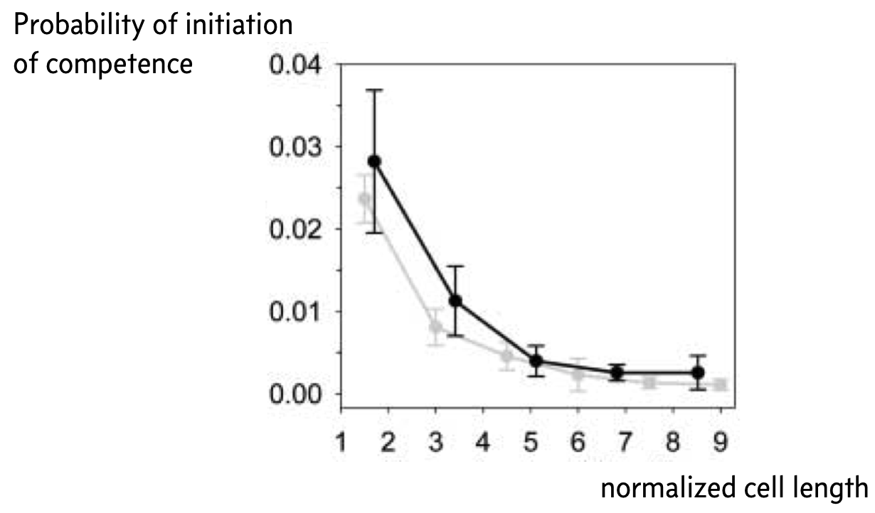
Remember that small copy numbers are a major source of noise. If we could make the copy numbers of the components of the competence circuit have higher copy numbers, we could reduce intrinsic noise. To accomplish this, Süel and coworkers used a ftsW mutant that fails to septate; that is, the cells do not divide. The result is long cells with high copy numbers.
Indeed, when they did this experiment, Süel and coworkers found that cells in their movies were less likely to become competent the longer, and therefore less noisy, the cell was, as shown in the figure below, taken from the 2007 paper. The black curve is from experimental measurements and the gray curve from analysis of stochastic simulations similar to what we show in the next section of this notebook. Here, the y-axis represents the probability that a given cell will become competent before division.
Tunable control of competence
A given cell may go in to competence before it divides. This depends on the amount of time it takes to get kicked into competence by intrinsic noise. Once competent, the cell may remain competent for a short or a long time. This depends on the dynamics as it traverses the competent loop of the phase portrait.
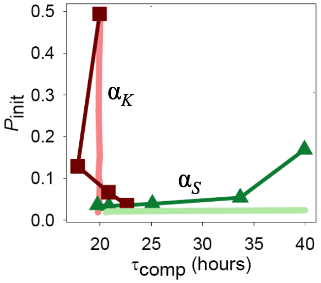
How can these two time scales, that is, the time scale to become competent and the time scale to return from competence, be tuned? Süel and coworkers found that these two time scales can be tuned independently by varying the constitutive expression of comK and comS, respectively, as parametrized by \(\alpha_k\) and \(\alpha_s\).
This stands to reason. If we make more ComK (increase \(\alpha_k\)), this pushes the circuit rightward in the phase portrait, into the competence loop. This results in shorter time to competence.
ComS must be degraded to allows the MecA complex to degrade ComK. So, the faster a cell can get rid of ComS, the faster it can degrade ComK and return from competence. So, if we increase \(\alpha_s\), more ComS is around, and competence is prolonged.
To study this quantitatively, we can take advantage of our ability to sample out of a probability distribution defined by a master equation. With samples, we can compute any quantity we like from them, including the amount of time before the circuit launches into competence and the amount of time it remains in competence. We need to modify some of the Gillespie simulation code to do this. First, we can code up the Gillespie draw, which is the same as in the chapter on the Gillespie SSA.
[49]:
@numba.njit
def gillespie_draw(propensities, population, t, args):
    """
    Draws a reaction and the time it took to do that reaction.
    """
    # Update propensities
    propensity(propensities, population, t, *args)

    # Sum of propensities
    props_sum = np.sum(propensities)

    # Compute time
    time = np.random.exponential(1 / props_sum)

    # Draw reaction given propensities
    rxn = biocircuits.gillespie._sample_discrete(propensities, props_sum)

    return rxn, time
With that in hand, we can code up a function that runs a Gillespie trajectory until competence is initialized (\(k\) goes above a threshold). It records that time, and then continues the trajectory, stopping when competence is exited (\(k\) goes below a threshold).
[50]:
@numba.njit
def competence_times(population_0, args, k_init=10000, k_back=7500, timeout=100000000.0):
    propensities = np.zeros(update.shape[0])
    population = population_0
    k = population[1]

    t = 0
    while t < timeout and k < k_init:
        event, dt = gillespie_draw(propensities, population, t, args)
        population += update[event, :]
        t += dt
        k = population[1]

    # Record time we entered competence
    t_init = t

    while t < timeout and k >= k_back:
        event, dt = gillespie_draw(propensities, population, t, args)
        population += update[event, :]
        t += dt
        k = population[1]

    # Record exit time of competence
    t_exit = t

    return t_init, t_exit
Now we’ll write a function to sample these times repeatedly. For each sample, we will first let the system settle around the stable fixed point in order to get an accurate value for the time to initiate competence. To do this, we will artificially expand the volume of the system using the parameter omega, since we already have seen that this reduces noise. We will then reset omega to its original level and draw the time scales of interest.
[51]:
def sample_competence_time(
    params_ssa,
    settle_time=504000,
    omega_scale=10,
    k_init=10000,
    k_back=7500,
    size=1,
    progress_bar=False,
):
    t_init = np.empty(size)
    t_comp = np.empty(size)

    iterator = tqdm.tqdm(range(size)) if progress_bar else range(size)
    for i in iterator:
        params_ssa_small_omega = params_ssa._replace(
            omega=params_ssa.omega / omega_scale
        )
        population_0 = np.array([10, 100, 10, 400, 500, 0, 0], dtype=int)
        time_points = np.linspace(0, 504000, 3)

        pop = biocircuits.gillespie_ssa(
            propensity,
            update,
            population_0,
            time_points,
            args=tuple(params_ssa_small_omega),
        )

        population_0 = pop[0, -1, :]
        t_init[i], t_exit = competence_times(population_0, tuple(params_ssa))

        t_comp[i] = t_exit - t_init[i]

    return t_init, t_comp
We are now set to do our calculations. We will vary \(\alpha_k\) against the “wild type” \(\alpha_k\) value; that is \(\alpha_k / \alpha_k^{\text{wild type}}\). We will vary the ration \(\alpha_s / \beta_s\). For both, we refer to the connections of the parameters for the discrete model compared to the continuous one. In practice, this means varying \(k_1\) and \(k_4\), respectively, for varying \(\alpha_k\) and \(\alpha_s\).
We will draw 100 samples of these times for each set of parameter values. We will store them in a Pandas DataFrame for convenience. Warning: If you are running this notebook, the following cell will take several minutes. If you want to speed up the calculation, you could run the Gillespie simulations in parallel.
[52]:
alpha_k_ratio = [1, 1.6, 2.5, 4, 6.3, 10]
alpha_s_ratio = [0.0, 0.02, 0.08, 0.15, 0.2, 0.25]
results = {
    "alpha_k_ratio": [],
    "alpha_s_ratio": [],
    "t_init": [],
    "t_comp": [],
}
size = 100

# Run calculations for varying alpha_k with alpha_s = 0
for akr in tqdm.tqdm(alpha_k_ratio):
    params_ssa_new = params_ssa._replace(k1=params_ssa.k1 * akr)
    t_init, t_comp = sample_competence_time(params_ssa_new, size=size)
    results["alpha_k_ratio"] += [akr] * size
    results["alpha_s_ratio"] += [
        params_ssa.k4
        / params_ssa.k5
        * params_ssa.P_comS_const
        / params_ssa.P_comS
    ] * size
    results["t_init"] = np.concatenate((results["t_init"], t_init))
    results["t_comp"] = np.concatenate((results["t_comp"], t_comp))

# Run calculations for varying alpha_s with alpha_k/alpha_k_wt = 1
for asr in tqdm.tqdm(alpha_s_ratio):
    k4 = asr * params_ssa.k5 * params_ssa.P_comS / params_ssa.P_comS_const
    params_ssa_new = params_ssa._replace(k4=k4)
    t_init, t_comp = sample_competence_time(params_ssa_new, size=size)
    results["alpha_k_ratio"] = np.concatenate(
        (results["alpha_k_ratio"], [1] * size)
    )
    results["alpha_s_ratio"] += [asr] * size
    results["t_init"] = np.concatenate((results["t_init"], t_init))
    results["t_comp"] = np.concatenate((results["t_comp"], t_comp))

df = pd.DataFrame(results)
100%|████████████████████████████████████████████| 6/6 [49:15<00:00, 492.62s/it]
100%|████████████████████████████████████████████| 6/6 [55:20<00:00, 553.44s/it]
For each of the plots, we can convert the time units from seconds to hours.
[53]:
df['time to competence (hr)'] = df['t_init'] / 3600
df['time competent (hr)'] = df['t_comp'] / 3600
Finally, we will display the plots as ECDFs, a type plot we encountered when discussing copy numbers in cells in our introduction to noise.
[54]:
plot_kwargs = dict(
    frame_height=200,
    frame_width=250,
    x_axis_type="log",
    style="staircase",
    x_range=[1, 2e4],
)

colors = bokeh.palettes.brewer['PuBu'][9]

plots = [
    [
        iqplot.ecdf(
            df.loc[df["alpha_s_ratio"] == 0, :],
            cats="alpha_k_ratio",
            q="time to competence (hr)",
            palette=colors,
            x_axis_label=None,
            **plot_kwargs,
        ),
        iqplot.ecdf(
            df.loc[df["alpha_s_ratio"] == 0, :],
            cats="alpha_k_ratio",
            q="time competent (hr)",
            palette=colors,
            x_axis_label=None,
            **plot_kwargs,
        ),
    ],
    [
        iqplot.ecdf(
            df.loc[df["alpha_k_ratio"] == 1, :],
            cats="alpha_s_ratio",
            q="time to competence (hr)",
            palette=colors,
            **plot_kwargs,
        ),
        iqplot.ecdf(
            df.loc[df["alpha_k_ratio"] == 1, :],
            cats="alpha_s_ratio",
            q="time competent (hr)",
            palette=colors,
            **plot_kwargs,
        ),
    ],
]

# Make legend titles
plots[0][0].legend.title = "αk/αk wt"
plots[1][0].legend.title = "αs/βs"
plots[0][1].legend.title = "αk/αk wt"
plots[1][1].legend.title = "αs/βs"

# Link x-axes
plots[1][0].x_range = plots[0][0].x_range
plots[1][1].x_range = plots[0][1].x_range

bokeh.io.show(bokeh.layouts.gridplot(plots))
The top row has \(\alpha_s\) fixed at zero, and the bottom row has \(\alpha_k/\alpha_k^{\text{wild type}}\) fixed at 1. The left column shows the ECDF of the time to initialize competence and the right columns show the ECDF of the time a cell remains competent. Note that the x-axis scale in all cases is logarithmic.
We will look at the plots one by one.
The upper left plot shows that as constitutive expression of ComK grows (\(\alpha_k\) increasing), the time it takes to initialize competence diminishes. Note, though, that the width of the ECDF grows with increasing time to competence. The coefficient of variation in time to competence grows from about 0.4 to 0.9 over the values of \(\alpha_k\) considered here. (This is calculated in the cell below.)
The upper right plot shows that while the time to initialize competence varies over two orders of magnitude, the amount of time that the cells remain competent is independent of \(\alpha_k\) in this regime.
The bottom right plot shows that increasing \(\alpha_s\) results in greater time in competence. The variation in time in a competent state also grows with increasing \(\alpha_s\), growing from 0.1 to 0.8 in this regime (calculated in a similar was as in the code cell below).
The bottom left plot shows that the time to initialize competence is more or less independent of \(\alpha_s\) in this regime.
Taken together, these results point to independent tuning of the time to initialize competence and the time spent in competence by the strength of constitutive expression of ComK and ComS, respectively. Indeed, Süel and coworkers found this to be the case experimentally. They made Bacillus strains that contains additional copies of comS or comK under control of inducible promoters so that they could artificially adjust \(\alpha_s\) and \(\alpha_k\). They then measured the time to competence and the time spent in competence and found that they could indeed be tuned independently.
Computing environment
[55]:
%load_ext watermark
%watermark -v -p numpy,scipy,numba,bokeh,iqplot,tqdm,biocircuits,jupyterlab
The watermark extension is already loaded. To reload it, use:
  %reload_ext watermark
Python implementation: CPython
Python version       : 3.9.12
IPython version      : 8.3.0

numpy      : 1.21.5
scipy      : 1.7.3
numba      : 0.55.1
bokeh      : 2.4.2
iqplot     : 0.2.3
tqdm       : 4.64.0
biocircuits: 0.1.8
jupyterlab : 3.3.2