Problem 9.1: Coupled repressilators
This problem is still a draft.
In this problem, we further study the dynamics of the repressilator, with the interesting twist that we will consider two coupled respressilators. A schematic of the repressilator is shown panel (a) of the figure below. Consider now two repressilators, which we will label x and y, that are coupled as in panel (b) of the figure below. For this coupling, we have chosen that gene A in the respective circuits repress their counterparts in the other. \(\mathrm{A}_\mathrm{x}\) and \(\mathrm{A}_\mathrm{y}\) have two repressors acting on them, and we assume if one or both of the repressors are bound (with their respective cooperativity), the polymerase is occluded.
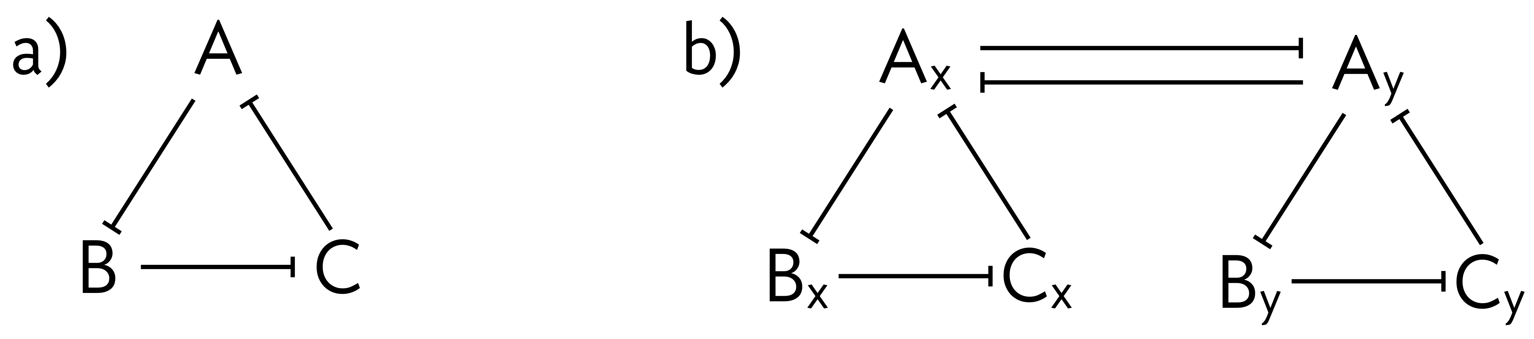
For simplicity, we will consider only the dynamics of the protein products and neglect the mRNA dynamics. We will further assume that each gene in the “x” repressilator has the same unregulated rate of production \(\beta_x\) and the same rate of dilution/decay, \(\gamma_x\). Each repressor acts on the other repressors within its repressilator with activation constant \(k\) and Hill coefficient \(n\). The same holds for the “y” repressilator; each gene has the same unregulated rate of production \(\beta_y\), the same rate of dilution/decay, \(\gamma_y\), and repress other genes within the “y” repressilator with Hill coefficient \(n\) and activation constant \(k\). We assume that the repressors in the “x” and the “y” repressilators have the same unregulated steady state level, which is to say that \(\beta_x/\gamma_x = \beta_y/\gamma_y\). Repression \textit{between} repressilators (in this case, A\(_\mathrm{x}\) repressing A\(_\mathrm{y}\) and A\(_\mathrm{y}\) repressing A\(_\mathrm{x}\)) operate with Hill coefficient \(n_c\) and activation constant \(k_c\).
a) Show that the dynamical equations of the circuit can be written in dimensionless form as
\begin{align} \dot{x}_a &= \frac{\beta}{1 + x_c^n + (\kappa y_a)^{n_c}} - x_a, \\ \dot{x}_b &= \frac{\beta}{1 + x_a^n} - x_b, \\ \dot{x}_c &= \frac{\beta}{1 + x_b^n} - x_c, \\ \gamma^{-1}\,\dot{y}_a &= \frac{\beta}{1 + y_c^n + (\kappa x_a)^{n_c}} - y_a, \\ \gamma^{-1}\,\dot{y}_b &= \frac{\beta}{1 + y_a^n} - y_b, \\ \gamma^{-1}\,\dot{y}_c &= \frac{\beta}{1 + y_b^n} - y_c. \end{align}
b) Show that if the two repressilators are completely uncoupled (achievable by setting \(\kappa = 0\)), the ratio of the periods of steady oscillation is \(T_x/T_y = \gamma\).
c) Numerically solve for the dynamics of the coupled repressilators. Use parameters \(n = 3\), \(n_c = 2\), \(\beta = 20\), \(\gamma = 3/2\). Solve for the dynamics both for \(\kappa = 0.1\) and \(\kappa = 1\) and generate plots. Comment on what you see.
d) Compute the period of steady oscillation for species \(\mathrm{B}_\mathrm{x}\) and \(\mathrm{B}_\mathrm{y}\) for the parameter values in part (c), but with \(\kappa\) ranging from zero to ten. Plot \(T_x\) and \(T_y\) versus \(\kappa\). Comment on the results. Specifically, comment on sychronization and where you see qualitative changes in the period as \(\kappa\) increases. Hint: There are many ways to compute the period of oscillation. You could use power
spectra, or you could detect where peaks are. To do the latter, the scipy.signal.argrelmax() function is useful.
e) This system is fun to play with. Invent another way to couple the represillators (i.e., change which species are coupled and whether or not the coupling is via repression or activation). Perform a similar set of analyses and comment on what you see.