The C1-FFL with AND logic has an on-delay, but no off-delay.
The C1-FFL with OR logic has an off-delay, but no on-delay.
The C1-FFL with both AND and OR logic can filter out short input impulses.
The I1-FFL with AND logic is a pulse generator and also speeds response compared to an unregulated circuit.
Concept
When multiple factors regulate a single gene, we need to specify the logic of the regulation, usually OR or AND.
Code
# Colab setup ------------------import os, sys, subprocessif"google.colab"in sys.modules: cmd ="pip install --upgrade colorcet biocircuits watermark" process = subprocess.Popen(cmd.split(), stdout=subprocess.PIPE, stderr=subprocess.PIPE) stdout, stderr = process.communicate()# ------------------------------import warningsimport numpy as npimport scipy.integrateimport biocircuitsfrom biocircuits.viz import bokeh_showwith warnings.catch_warnings(): warnings.simplefilter("ignore", category=SyntaxWarning)import biocircuits.appsimport colorcetcolors = colorcet.b_glasbey_category10import bokeh.ioimport bokeh.layoutsimport bokeh.modelsimport bokeh.plotting# Set to True to have fully interactive plotsinteractive_python_plots =Falsenotebook_url ="localhost:8888"bokeh.io.output_notebook()
Loading BokehJS ...
4.1 Finding 3-gene motifs in a bacterial transcriptional network
After three chapters, we have developed a toolbox of numerical, analytical, and plotting-based approaches, and applied them to various single-gene and two-gene circuits. In the last chapter, we discussed a toggle switch that generates bistability via mutual repression by two repressor proteins. We will now move on to systems with more components and greater functional complexity, starting with three-component circuits.
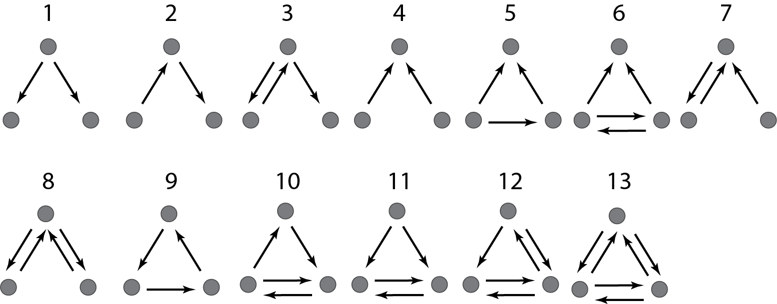
There are thirteen different ways in which three transcription factors can regulate one another, as diagrammed below. Which ones should we analyze first? A sensible choice is to again look toward natural gene regulatory networks and ask which of these potential circuits are overrepresented in natural circuits, i.e. which (if any) of these are network motifs, which are, as a reminder, statistically over-represented circuits in natural networks (circuits).
{$fig-all-three-node-motifs-milo width=400px}
Milo and coworkers ((Milo et al. 2002)) performed just such an analysis. The authors then tabulated the number of times that each of these thirteen regulatory patterns in maps of natural transcriptional circuits. But a question remains: How often would one expect to see any one of these given patterns within a circuit of that size? In order to answer this question, a null model for a network is required. We hinted at this concept in Chapter 2, and here we go into more detail.
4.2 Random graphs enable motif identification
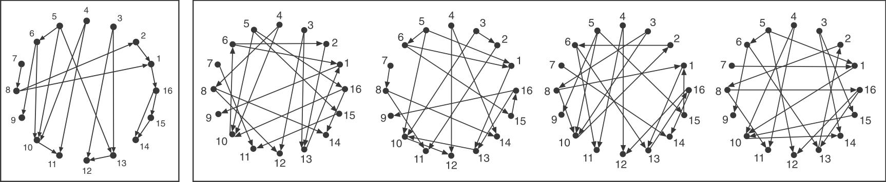
Consider a directed graph representing a hypothetical regulatory circuit (left). As before, each numbered node in this network represents an operon or transcription factor, and arrows indicate regulation of the target node by a transcription factor in the source node. To find over-represented patterns in this graph, we can compare it to an ensemble of randomized variants and look for sub-graphs that occur more frequently in the real circuit than in the random variants.
Figure 4.1: Schematic comparison between a specific circuit (left) and a set of randomized variants with the same incoming and outgoing arrow distributions (right). Image modified from (Milo et al. 2002)
To make the comparison as fair as possible, we need to design variant graphs that maintain the key statistical properties of the original graph. Specifically, we insist that all variant graphs have the same number of nodes and arrows. But this is not really enough: It would not make sense to compare a graph whose arrows are distributed over all the nodes to a variant in which, say, all arrows stem from a single source node, or converge on a single target node. We therefore need to impose a stronger constraint: all variant graphs should maintain the exact distribution of incoming and outgoing arrows for each node.
If you examine the graphs above, you can see that they were constructed to have the same numbered nodes. Furthermore, the number of arrows exiting and entering each numbered node is exactly the same in all graphs. For example, node 4 always has 2 outgoing arrows. Node 6 always has one incoming and two outgoing arrows, node 12 always has 2 incoming arrows, and so on.
To generate the randomized graphs, imagine cutting each arrow in half with a scissors to generate a dangling “+” end connected to an arrowhead and a dangling “–” end connected to a source node. Then imagine tying each “+” end to a randomly chosen “–” end. Voila, we have a new randomized graph, guaranteed through this procedure to maintain the same joint distribution of incoming and outgoing arrows. For more details, see the algorithms in (Shen-Orr et al. 2002) and in (Newman et al. 2001).
4.2.1 The feedforward loop is overrepresented in natural transcriptional networks
Now that we understand how to formulate a proper null model for motif identification, we return to the analysis by Milo, et al. The authors used a z-score to quantify over- or under-representation in units of the standard deviation of the number of occurrences for the sub-graph in the randomized circuits,
\[
\begin{align}
z = \frac{n_{obs}-\langle n\rangle}{\sigma},
\end{align}
\tag{4.1}\]
where \(n_{obs}\) is the number of times the sub-graph was observed in the actual circuit, \(\langle n\rangle\) is the mean number of times it was observed in randomized circuits, and \(\sigma = \sqrt{\langle (n-\langle n \rangle)^2\rangle}\) is the standard deviation of the number of times it was observed in randomized circuits. For comparison purposes, Milo and coworkers defined a normalized z-score. Considering the z-score of sub-graph \(i\), the normalized z-score is
They did this for several transcriptional circuits, including E. coli, yeast (two versions), and B. subtilis. In the plot below (data digitized from (Milo et al. 2004)), the four networks are so similar in their normalized z-score profiles that the different organisms overlap almost perfectly.
Figure 4.2: z-scores for all three node motifs in various species. Data digitized from [milo:2004a].
As you can see, one particular motif, number 5, is overrepresented in all of the transcriptional networks, number 7:
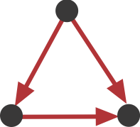
Figure 4.3: FFL motif
This sub-graph, termed the feed-forward loop (FFL), has one node that regulates a target node two ways: directly, and indirectly through the third node.
Several features are striking from their results:
There is strong over-representation of feed-forward loops (FFLs). In E. coli, one expects to see 7±5 FFLs by chance, but one observes this pattern 42 times in the real circuit.
The over-representation of FFLs is conserved across three distinct organisms, suggesting it is a general property of transcriptional circuits.
Most other sub-graphs are neither over- nor under-represented.
Three sub-graphs are statistically under-represented. They occur significantly less often than one would expect by chance, provoking the question of what problems they might present as components of larger circuits. These three sub-graphs are all sub-graphs of the FFL sub-graph. Thus, it is not that, e.g., divergent regulation (represented by sub-graph 1) is rare; it is just that when it does occur, it does so in the context of the FFL.
4.3 There are many kinds of FFLs
Our description of regulatory interactions in the FFL so far has been oversimplified in several ways:
We have not distinguished between positive regulation (activation) and negative regulation (repression).
We have not considered how multiple regulators combine to control expression of a mutual target operon.
We have ignored the quantitative aspects of regulation.
Understanding the biological function of a motif requires thinking about these aspects more carefully.
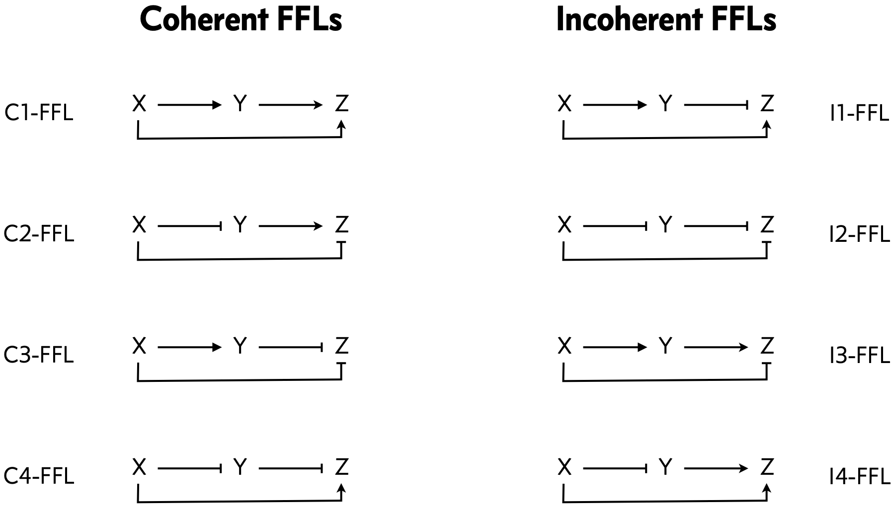
To address the first point, we can classify the overall FFL motif into \(2^3=8\) different categories depending on which of its 3 arrows are positive or negative:
Figure 4.4: FFL classes
In this classification, half of the FFL architectures are coherent, meaning that X’s direct regulation of Z and its indirect regulation of Z are of the same type, both activating or both repressing. the other half are incoherent, meaning that the direct and indirect regulatory paths have the opposite sign.
We can further sub-classify the FFLS, according to how the regulatory arrows converging on the third node (now labeled “Z”) combine. Consider first the example where both X and Y activate Z, as in the C1-FFL and I4-FFl. In AND regulation, both X and Y need to be simultaneously present at high levels for Z to be expressed. In OR regulation, either input being at a high level is sufficient to activate Z. We will discuss this logic in more detail momentarily in Section 4.5.
Now that we have defined what FFLs are and how we can represent them, we will spend the rest of this chapter (and even some beyond) considering what functions the various FFLs can perform for cells.
4.4 The most-encountered FFLs
While FFLs in general are motifs, some FFLS are more often encountered than others. In the figure below, using data taken from (Alon 2007), we see relative abundance of the eight different FFLs in E. coli and S. cerevisiae. Two FFLs, C1-FFL and I1-FFL, stand out as having much higher abundance than the other six. We will focus our study on these two in this chapter.
4.5 Logic of regulation by two transcription factors
Because X and Y both regulate Z in an FFL, we need to specify how they collaborate in the regulation.
For the sake of illustration, let us assume we are discussing C1-FFL, where X activates Z and Y also activates Z. One can imagine a scenario where both X and Y need to be present to turn on Z. For example, they could be binding partners that together serve to recruit polymerase to the promoter. We call this AND logic. In other words, to get expression of Z, we must have X AND Y. Conversely, if either X or Y may each alone activate Z, we have OR logic. That is, to get expression of Z, we must have X OR Y.
So, to fully specify an FFL, we need to also specify the logic, either AND or OR, of how Z is regulated. Including choice of logic gives a total of 16 possible FFLs.
We are now left with the task of figuring out how to mathematically encode AND and OR logic. Before doing so, we note that, as discussed previously, we are using Hill functions, which are phenomenological functions describing how effectors may regulate gene expression capturing both the necessary concentration of effector (\(k\)) and the ultrasensitivity of the regulation (\(n\)). When the molecular details of the regulation mechanics of an effector are known, we may derive the appropriate functions describing gene expression regulation rather than using Hill function. Similarly, for two effectors, we could also derive the functions from the molecular details and discover what kind of logic emerges. See, for example, (Bintu et al. 2005). We often do not know the molecular details, and Hill functions and the two-effector variants thereof we present below are quite useful in analyzing the properties of circuit architectures.
We now proceed to formally write mathematical expressions for the dynamics of a gene product Z under regulatory control of effectors X and Y. The dynamics of the concentration of Z may be written as
where the lowercase letters denote the concentrations of the respective species.
Our goal is to specify the dimensionless regulatory function \(f(x, y)\) that encodes how X and Y may together regulate Z. Our approach is to assign a “weight” to each state of a promoter region. With two effectors, X and Y, the promoter region could be unbound, bound with X, bound with Y, or bound with both X and Y. To get the regulatory function, we sum the weights of states that allow polymerase binding and divide by the sum of all weights. This gives the fraction of time that expression of the gene is “on.” For example, if X and Y are both activators and they together have AND logic, we have
\[
\begin{align}
f(x, y) = \frac{\text{X and Y bound weight}}{(\text{unbound weight}) + (\text{X bound weight}) + (\text{Y bound weight}) + (\text{X and Y bound weight})}
\end{align}
\tag{4.4}\]
The weights are chosen to give Hill-like functions.
promoter region state
weight
dimensionless weight
unbound
\[1\]
\[1\]
X bound
\[(x/k_x)^{n_x}\]
\[x^{n_x}\]
Y bound
\[(y/k_y)^{n_y}\]
\[y^{n_y}\]
X and Y bound
\[(x/k_x)^{n_x}\,(y/k_y)^{n_y}\]
\[x^{n_x}\,y^{n_y}\]
The dimensionless weights are given by substituting \(x \leftarrow x/k_x\) and \(y \leftarrow y/k_y\). We will use the dimensionless versions of these functions henceforth. We note that the denominator of the regulatory function \(f(x,y)\) is always the same,
Alternatively, we could have a structure where maximally only one of the two effectors may be bound at a time (for example due to steric reasons), in this case the states and weights are given in the table below.
promoter region state
weight
dimensionless weight
unbound
\[1\]
\[1\]
X bound
\[(x/k_x)^{n_x}\]
\[x^{n_x}\]
Y bound
\[(y/k_y)^{n_y}\]
\[y^{n_x}\]
In this case, the denominator for all of the regulatory functions is \(1 + x^{n_x} + y^{n_y}\). We will refer to such regulatory functions as corresponding to “single occupancy.”
With this prescription, let us proceed to write the regulatory functions \(f(x, y)\) for various architectures.
4.5.1 Logic with two activators
Let us start first with X and Y, both activating, with AND logic, as seen in the C1-FFL and I4-FFL. To help conceptualize how the logic translates into expression of Z before we get into the mathematical expressions, we can construct a truth table for whether or not Z is on, given the on/off status of X and Y. The truth table is shown below, with a zero entry meaning that the gene is not on and a one entry meaning it is on.
X
Y
Z
0
0
0
0
1
0
1
0
0
1
1
1
We can also construct a truth table for OR logic with X and Y both activating.
X
Y
Z
0
0
0
0
1
1
1
0
1
1
1
1
Following the above prescription, the dimensionless regulatory functions are
We can make plots of these regulatory functions to demonstrate how they represent the respective logic. To accentuate the logic, we will choose very sharp Hill functions \(n_x = n_y = 20\).
Figure 4.6: Illustration of activating Hill functions with various logic.
Here, purple indicates that \(f(x, y)\) is zero and yellow indicates that \(f(x, y)\) is one. With AND logic, both X and Y must have high concentrations for Z to be expressed. Conversely, for OR logic, X or Y or both can be in high concentrations for Z to be expressed, but if neither is high enough, Z does not get expressed. These graphical representations of the mathematical expressions for regulation indeed match the conceptual truth tables we started with.
4.6 Logic with two repressors
Now let’s consider the case where we have two repressors, as in the C3-FFL or I2-FFL. The AND case where X and Y are both repressors is NOT X AND NOT Y.
X
Y
Z
0
0
1
0
1
0
1
0
0
1
1
0
Here, either repressor (or both) can shut down gene expression.
For OR logic with two repressors, we have NOT X OR NOT Y. Its truth table is below.
X
Y
Z
0
0
1
0
1
1
1
0
1
1
1
0
We might get this kind of logic if the two repressors need to work in concert, perhaps through binding interactions, to affect repression.
We can encode these two truth tables with dimensionless regulation functions
Figure 4.7: Illustration of repressive Hill functions with various logic.
4.6.1 Logic with one activator and one repressor
Now say we have one activator (which we will designate to be X) and one repressor (which we will designate to be Y). Now, AND logic means X AND NOT Y, and OR logic means X OR NOT Y. The truth table for the AND gate is below.
In the single occupancy case, once levels of both X and Y exceed unity (or their Hill activitation constants in dimensional units), the relative levels of the respective genes become important. Gene expression is on if Y is not too high relative to X.
Figure 4.8: Illustration of Hill functions for one activator and one repressor with various logic.
4.6.2 Connection to logic gates
When two “input” effectors regulate the expression of a single “output” gene, we are tempted to connect the circuit architectures to logic gates. This is both useful and dangerous.
First, we will discuss the utility. Boolean algebra is a very powerful tool in developing circuits in digital electronics, and may also be a powerful framework for designing biological circuits. Briefly, Boolean algebra deals with only trues and falses, or ones and zeros. It has three fundamental operations, conjuction (∧), disjunction (∨), and negation (¬). They are defined such that
One could think of two activators X and Y regulating expression of a gene Z with AND logic as Z = X ∧ Y. The relation X ∧ Y has a name; it is called an AND gate. The other architectures also represent logic gates. Below is a table of the analogous logic gates and Boolean algebra expressions for the two-effector regulation architectures we have considered.
X
Y
regulatory logic
idealized logic gate
Boolean algebra
activator
activator
AND
AND
X ∧ Y
activator
activator
OR
OR
X ∨ Y
repressor
repressor
AND
NOR
¬X ∧ ¬Y = ¬(X ∨ Y)
repressor
repressor
OR
NAND
¬X ∨ ¬Y = ¬(X ∧ Y)
activator
repressor
AND
NIMPLY
X ∧ ¬Y
activator
repressor
OR
IMPLY*
X ∨ ¬Y
*An IMPLY gate has a Boolean algebraic representation of ¬X ∨ Y, which we would get if we had arbitrarily chosen X to be the repressor instead of Y.
Now, let’s consider the danger in using digital logic with these circuits. While thinking digitally for these circuits has its merit (indeed, we used a giant Hill coefficient in making the images above showing the expression levels of Z as a function of X and Y concentration), we must always remember that biological circuits are more fuzzy. As an example, let’s look at how the one repressor/one activator system looks with a Hill coefficient of two.
Figure 4.9: Illustration of Hill functions for one activator and one repressor with a Hill coefficient of two with various logic.
This looks a lot less digital!
We are also limited by physiological realities in our use of the Hill-like function to descibe the regulatory functions of all two-input gates we can make with Boolean logic. You may notice that we are missing XOR (exactly one of X or Y is high to give high Z) and XNOR (X and Y are either both high or both low to give high Z), the two other basic two-input logic gates. We leave it to the reader to work out what the Hill-like regulatory functions \(f(x,y)\) for these gates would be following the prescription we have been using. Also think about how XOR- or XNOR-like logic might occur physiologically and why we usually do not use the Hill-like functions we are employing here in those cases. You can explore these ideas in an exercise.
4.7 Regulatory functions and their derivatives
As we proceed through analysis of biological circuits, we will use the regulatory functions we have just derived, in addition to activating and repressive Hill functions, extensively. For convenience, these functions and their derivatives with respect to \(x\) and \(y\) are in Appendix D.
4.8 The biocircuits package and regulatory functions
The biocircuits package contains the regulatory functions we have just described. The available regulatory functions and call signatures are:
Repressive Hill function: biocircuits.rep_hill(x, n)
Activating Hill function: biocircuits.act_hill(x, n)
Two activators with AND logic: biocircuits.aa_and(x, y, nx, ny)
Two activators with OR logic: biocircuits.aa_or(x, y, nx, ny)
Two activators with AND logic, single occupancy: biocircuits.aa_or_single(x, y, nx, ny)
Two repressors with AND logic: biocircuits.rr_and(x, y, nx, ny)
Two repressors with OR logic: biocircuits.rr_or(x, y, nx, ny)
Two repressors with AND logic, single occupancy: biocircuits.rr_and_single(x, y, nx, ny)
One activator and one repressor with AND logic: biocircuits.ar_and(x, y, nx, ny)
One activator and one repressor with OR logic: biocircuits.ar_or(x, y, nx, ny)
One activator and one repressor with AND logic, single occupancy: biocircuits.ar_and_single(x, y, nx, ny)
One activator and one repressor with OR logic, single occupancy: biocircuits.ar_or_single(x, y, nx, ny)
It is important to note that the inputs x and y are dimensionless. In the case of one activator and one repressor, x is always assumed to the the concentration of the activator and y that of the repressor.
The code comprising the functions are simply expressions of the mathematical equations given above using Numpy arrays. For example, the contents of biocircuits.rr_and() is given below.
def rr_and(x, y, nx, ny):"""Dimensionless production rate for a gene regulated by two repressors with AND logic in the absence of leakage. Parameters ---------- x : float or NumPy array Concentration of first repressor. y : float or NumPy array Concentration of second repressor. nx : float Hill coefficient for first repressor. ny : float Hill coefficient for second repressor. Returns ------- output : NumPy array or float 1 / (1 + x**nx) / (1 + y**ny) """return1/ (1+ x ** nx) / (1+ y ** ny)
These functions were used in generating the plots above, and we will use them going forward in this chapter as we numerically evaluate the dynamical equations of FFLs and beyond.
4.9 Dynamical equations for FFLs
To analyze the C1-FFL (or any of the other FFLs), in response to changes in the input X, we can write a generic system of ODEs for the concentrations of Y and Z. We know that Y is either activated or repressed by X and itself experiences degradation. We define a dimensionless function \(f_y(x/k_{xy}; n_{xy})\) to describe the activating or repressive Hill function for the regulation of X by Y. We have used the notation that \(n_{ij}\) is the Hill coefficient for j regulated by i, with \(k_{ij}\) similarly defined. To be explicit, if X activates Y, then
Similarly, we define the dimensionless function \(f_z(x/k_{xz}, y/k_{yz}; n_{xz}, n_{yz})\) to describe the regulation in expression of Z by X and Y. This have any of the functional forms we have listed above for activation/repression pairs and AND/OR logic. The dynamical equation for \(z\) is then
We can nondimensionalize these equations by choosing
\[
\begin{align}
t &= \tilde{t} / \gamma_y, \\[1em]
x &= k_{xz}\,\tilde{x},\\[1em]
y &= k_{yz}\,\tilde{y},\\[1em]
z &=z_d\,\tilde{z},
\end{align}
\tag{4.17}\]
where \(z_d\) is as of yet unspecified. Inserting these expressions into the dynamical equations gives
In addition to the Hill coefficients, these dimensionless parameters complete the parameter set of a dynamical system describing an FFL. Each has a physical meaning. The parameter \(\beta\) is the dimensionless unregulated steady state level of \(y\), \(\gamma\) is the ratio of the decay rates of Z and Y, and \(\kappa\) is the ratio of the amounts of X that are necessary to regulate Z and Y.
Henceforth, we will work with these dimensionless equations and will drop the tildes for notational convenience.
Note that these are dynamical equations for any FFL. It is not much more difficult to consider numerical solutions of all FFLs than one individually, so we develop functions in the technical appendix for that purpose. The functions are available in the biocircuits.apps module.
4.10 The C1-FFL circuit enables sign-sensitive delay
Now that we have laid the computational groundwork, we will proceed to an analysis of the first of the two over-represented FFLs, the C1-FFL. For reference, here again are the dimensionless dynamical equations:
Now, let us look at the dynamics for a sudden step up and step down in X. We will use dimensionless parameter values \(\beta = 5\), \(\gamma = \kappa = 1\), \(n_{xy} = n_{yz} = 3\), and \(n_{xy} = 5\).
Figure 4.10: Response of a C1-FFL with AND logic to a step up-and-down input.
Notice that there is a time delay for production of Z upon stimulation with X. This is a result of the AND logic. Though X has immediately come up, we have to wait for the signal to pass through Y for Z to come up. However, there is no delay when the signal X is turned off. The z curve responds immediately. This off-response is perhaps more apparent if we normalize the concentrations.
Figure 4.11: Normalized response of a C1-FFL with AND logic to a step up-and-down input.
Here, the on-delay is more apparent, as is the fact that both Y and Z have their levels immediately decrease when the X stimulus is removed. So, we have arrived at a design principle: The C1-FFL with AND logic has an on-delay, but no off-delay.
4.10.1 The magnitude of the delay can be tuned with κ
How might we get a longer delay? If we decrease \(\kappa = k_{xz}/k_{yz}\), we are increasing the disparity between the threshold levels needed to turn on gene expression. This should result in a longer time delay. Let’s try it for \(\kappa = 0.1\).
Figure 4.12: Response of a C1-FFL with AND logic to a step up-and-down input with \(\kappa = 0.1\).
Indeed, the delay is longer with small κ. We can quantify how the delay changes with κ by plotting how long it takes for the \(z\) level to rise to ten percent of its steady state value for various values of κ.
Code
tau = []kappa_vals = np.logspace(-1, 2, 200)# Finer time pointst_ = np.linspace(0, 20, 5000)for kappa in kappa_vals:# Solve for the dynamics yz = biocircuits.apps.solve_ffl( beta, gamma, kappa, n_xy, n_xz, n_yz, "c1", "and", t_, np.inf, 1 )# Determine threshold value z_thresh = yz[-1, 1] *0.1# Find where the threshold is crossed tau.append(t_[np.searchsorted(yz[:,1], z_thresh)])p = bokeh.plotting.figure( frame_width=400, frame_height=250, x_axis_type="log", x_axis_label="κ", y_axis_label="time to 10% of steady state", x_range=[0.1, 100], y_range=[0, 1.25],)p.scatter(kappa_vals, tau)bokeh_show(p)
Figure 4.13: Dependence of the response time of a C1-FFL with AND logic on the parameter \(\kappa\).
The delay does not change substantially, only about a factor of three over many orders of magnitude of κ.
4.10.2 The delay does not require ultrasensitivity
We might think that ultrasensitivity is required for the delay, but it is not, as seen by the calculation below with \(n_{xy} = n_{xz} = n_{yz} = 1\).
Figure 4.14: Response of a C1-FFL with AND logic to a step up-and-down input in the absence of ultrasensitivity.
Without ultrasensitivity, the delay is shorter, but present nonetheless. This is because with AND logic, the expression of Z still has to wait for Y to get high enough to begin producing Z at an appreciable level, regardless of how ultrasensitive the dynamics are.
4.10.3 The C1-FFL with AND logic and filter out short pulses
Now, let’s see what happens if we have a shorter pulse. The delay feature of the C1-FFl should filter out pulses that are shorter than the time scale of the delay.
Figure 4.16: Response of a C1-FFL with OR logic to a step up-and-down input.
Now we see that both Y and Z immediately start being produced upon stimulus, but there is a delay in the decrease of Z when the stimulus is removed. As with the AND logic, this is perhaps more easily seen with normalized concentrations.
Figure 4.17: Normalized response of a C1-FFL with OR logic to a step up-and-down input.
The level of Z in a C1-FFL with OR logic does respond to a pulse in X, but, analogously to the case with AND logic, it ignores a quick decrease and increase in X. We will not show that calculation here, but encourage you to do it yourself or explore that scenario with the dashboard below.
4.10.5 Sign sensitive delay is observed experimentally
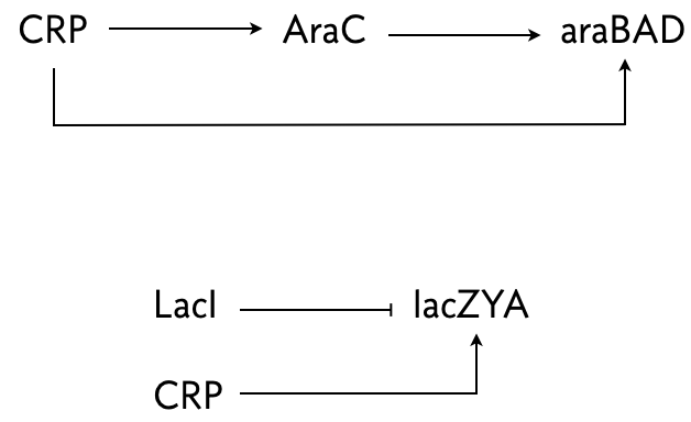
The arabinose and lac systems in E. coli are both turned on by cyclic AMP (cAMP), which stimulates production of CRP, but they have different architectures, shown below.
Figure 4.18: araBAD and lacZYA
In both systems where multiple species regulate one, AND logic is employed.
Mangan an coworkers (Mangan et al. 2003) performed an experiment where they put a fluorescent reporter under control of the products of these two systems, araBAD and lacZYA, respectively. In the lac system, IPTG was also present, so LacI was inhibited. Thus, lacZYA production was directly activated by CRP. Conversely, the arabinose system is a C1-FFL.
They measured the fluorescent intensity in cells that were suddenly exposed to cAMP. The response of these two systems to the sudden jump in cAMP is shown in the left plot below.
While the lac system responds immediately, the arabinose system exhibits a lag before responding. This is indicative of a time delay for a step on in the stimulus for a C1-FFL. Conversely, after these systems come to steady state and are subjected to a sudden decrease in cAMP, both the arabinose and lac systems respond immediately, without delay, which is also expected from a C1-FFL with AND logic.
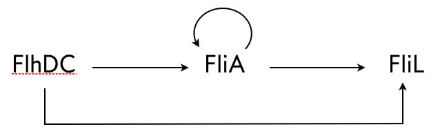
Kalir and coworkers ((Kalir et al. 2005)) did a similar experiment with another C1-FFL circuit found in E. coli, this time with OR logic. A circuit that regulates flagella formation is a “decorated” C1-FFL, shown below. We say it is decorated because the “Y” gene, in this case FliA, is also autoregulated. Importantly, the regulation of FliL by FliA and FlhDC is governed by OR logic.
Figure 4.20: Schematic drawing of the fliA system
Kalir and coworkers used engineered cells in which the FlhDC gene was under control of a promoter which could be induced with L-arabinose, a chemical inducer. The gene product FliL was altered to be fused to GFP to enable fluorescent monitoring of expression levels. To consider a circuit where FlhDC directly activates FliL, Kalir and coworkers used mutant E. coli cells in which the fliA gene was deleted.
Because of the OR logic, we would expect that a sudden increase in FlhDC would result in both the wild type and mutant cells to respond at the same time, that is with no delay. Fluorescence traces from these experiments are shown in the left plot, below.
Both strains show a delay, which is due to waiting for FlhDC to be activated, but both come on at the same time. Conversely, after the inducer is removed and FlhDC levels go down, the system with the wild type C1-FFL circuit shows a delay before the FliL levels drop off, while the mutant does not. This demonstrates the sign-sensitivity with OR logic.
4.11 The I1-FFL with AND logic is a pulse generator
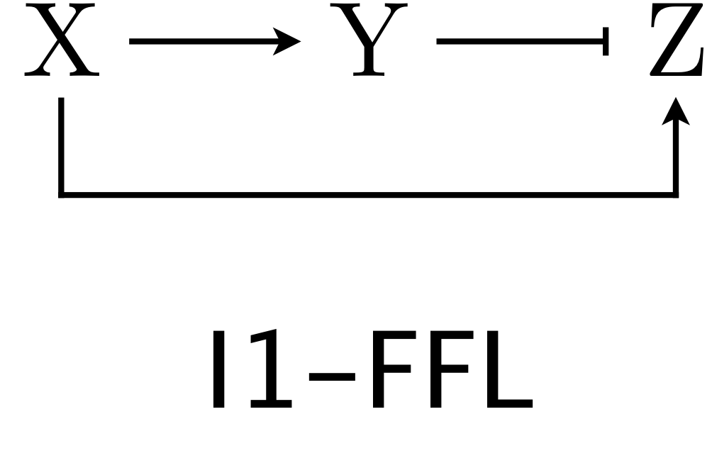
We now turn our attention to the other over-represented circuit, the I1-FFL. As a reminder, here is the structure of the circuit.
FFL abundance
X activates Y and Z, but Y represses Z. We can use the expressions for production rate under AND and OR logic for one activator/one repressor that we showed above in writing down our dynamical equations. Here, we will consider AND logic. The dimensionless dynamical equations are
In our first analysis of this circuit, we will investigate the response in Z to a sudden, sustained step in stimulus X. We will choose \(\gamma = 10\), which means that the dynamics of Z are faster than Y.
Figure 4.22: Demonstration of an I1-FFL with AND logic as a pulse generator.
We see that Z pulses up and then falls down to its steady state value. This is because the presence X leads to production of Z due to its activation. X also leads to the increase in Y, and once enough Y is present, it can start to repress Z. This brings the Z level back down toward a new steady state where the production rate of Z is a balance between activation by X and repression by Y. Thus, the I1-FFL with AND logic is a pulse generator.
4.11.1 The I1-FFL with AND logic gives an accelerated response
Let us compare the response of an I1-FFL being suddenly turned on (by a step in X) to an unregulated circuit that achieves the same steady state. Recall that the dimensionless dynamics for the unregulated circuit (that is, X ⟶ Z, the circuit in the absence of Y) follow
If we plot the normalized I1-FFL together with the unregulated response, we see that the I1-FFl makes it to the steady state faster, though it overshoots and then relaxes.
Figure 4.23: Demonstration of the fast response time of an I1-FFL with AND logic.
So, we have another design principle, The I1-FFL with AND logic has a faster response time than an unregulated circuit.
4.11.2 The accelerated response of the I1-FFL is observed experimentally
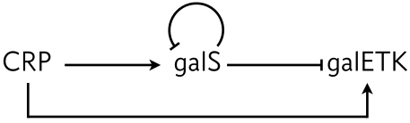
Mangan and coworkers (Mangan et al. 2006) investigated an I1-FFL circuit that E. coli uses in its galactose utilization system. The circuit is shown below.
Figure 4.24: Schematic of the gal E system
As the “X” gene in this I1-FFL is CRP, the circuit is induced by sudden addition of cAMP, as in the arabinose and lactose circuits above. Mangan and coworkers investigated the response of the wild type circuit, as well as a mutant circuit where galS was deleted. This latter circuit lacks the feed forward loop, and the production of galETK is directly regulated by CRP.
In their experiment, the galE promoter was engineering to express GFP so they could monitor the dynamics of the circuit with fluorescence. The result is shown below.
We see that indeed the wild type I1-FFL architecture speeds up the response to the cAMP input, complete with the overshoot we expect from an I1-FFL circuit.
4.12 A dashboard for exploring FFLs
The biocircuits package has apps to explore properties of some specific circuits. To explore FFLs, you and use the FFL app. (The apps submodule of biocircuits must be imported separately.) You can use this app to explore how the C1-FFL and I1-FFL studied in this chapter responds to steps up and down in input. You can also explore the dynamics of the other six FFLs. We encourage you to look at the code in the biocircuits package that generates the app so you can see how the dashboard is build.
Note that if you are viewing the code cell below in the static HTML rendering of this notebook, it will not appear.
if interactive_python_plots: app = biocircuits.apps.ffl_app() bokeh.io.show(app, notebook_url=notebook_url)
Alon, Uri. 2007. “Network Motifs: Theory and Experimental Approaches.”Nature Reviews Genetics 8 (6): 450–61. https://doi.org/10.1038/nrg2102.
Bintu, Lacramioara, Nicolas E. Buchler, Hernan G. Garcia, et al. 2005. “Transcriptional Regulation by the Numbers: Models.”Current Opinion in Genetics & Development 15 (2): 116–24. https://doi.org/10.1016/j.gde.2005.02.007.
Kalir, Shiraz, Shmoolik Mangan, and Uri Alon. 2005. “A Coherent Feed-Forward Loop with a SUM Input Function Prolongs Flagella Expression in Escherichia Coli.”Molecular Systems Biology 1: 2005.0006. https://doi.org/10.1038/msb4100010.
Mangan, Shmoolik, Shalev Itzkovitz, Alon Zaslaver, and Uri Alon. 2006. “The Incoherent Feed-Forward Loop Accelerates the Response-Time of the Gal System of Escherichia Coli.”Journal of Molecular Biology 356 (5): 1073–81. https://doi.org/10.1016/j.jmb.2005.12.003.
Mangan, Shmoolik, Alon Zaslaver, and Uri Alon. 2003. “The Coherent Feedforward Loop Serves as a Sign-Sensitive Delay Element in Transcription Networks.”Journal of Molecular Biology 334 (2): 197–204. https://doi.org/10.1016/j.jmb.2003.09.049.
Milo, Ron, Shalev Itzkovitz, Nadav Kashtan, et al. 2004. “Superfamilies of Evolved and Designed Networks.”Science 303 (5663): 1538–42. https://doi.org/10.1126/science.1089167.
Milo, Ron, Shai Shen-Orr, Shalev Itzkovitz, Nadav Kashtan, Dmitri Chklovskii, and Uri Alon. 2002. “Network Motifs: Simple Building Blocks of Complex Networks.”Science 298 (5594): 824–27. https://doi.org/10.1126/science.298.5594.824.
Newman, Mark E. J., Steven H. Strogatz, and Duncan J. Watts. 2001. “Random Graphs with Arbitrary Degree Distributions and Their Applications.”Physical Review E 64 (2): 026118. https://doi.org/10.1103/PhysRevE.64.026118.
Shen-Orr, Shai S., Ron Milo, Shmoolik Mangan, and Uri Alon. 2002. “Network Motifs in the Transcriptional Regulation Network of Escherichia Coli.”Nature Genetics 31 (1): 64–68. https://doi.org/10.1038/ng881.

 {$fig-all-three-node-motifs-milo width=400px}